CHAPTER 11 Caching and file systems

The cache manager is a set of kernel-mode functions and system threads that cooperate with the memory manager to provide data caching for all Windows file system drivers (both local and network). In this chapter, we explain how the cache manager, including its key internal data structures and functions, works; how it is sized at system initialization time; how it interacts with other elements of the operating system; and how you can observe its activity through performance counters. We also describe the five flags on the Windows CreateFile function that affect file caching and DAX volumes, which are memory-mapped disks that bypass the cache manager for certain types of I/O.

The services exposed by the cache manager are used by all the Windows File System drivers, which cooperate strictly with the former to be able to manage disk I/O as fast as possible. We describe the different file systems supported by Windows, in particular with a deep analysis of NTFS and ReFS (the two most used file systems). We present their internal architecture and basic operations, including how they interact with other system components, such as the memory manager and the cache manager.

The chapter concludes with an overview of Storage Spaces, the new storage solution designed to replace dynamic disks. Spaces can create tiered and thinly provisioned virtual disks, providing features that can be leveraged by the file system that resides at the top.

Terminology

To fully understand this chapter, you need to be familiar with some basic terminology:

• ■    Disks are physical storage devices such as a hard disk, CD-ROM, DVD, Blu-ray, solid-state disk (SSD), Non-volatile Memory disk (NVMe), or flash drive.

• ■    Sectors are hardware-addressable blocks on a storage medium. Sector sizes are determined by hardware. Most hard disk sectors are 4,096 or 512 bytes, DVD-ROM and Blu-ray sectors are typically 2,048 bytes. Thus, if the sector size is 4,096 bytes and the operating system wants to modify the 5120th byte on a disk, it must write a 4,096-byte block of data to the second sector on the disk.

• ■    Partitions are collections of contiguous sectors on a disk. A partition table or other disk-management database stores a partition’s starting sector, size, and other characteristics and is located on the same disk as the partition.

• ■    Volumes are objects that represent sectors that file system drivers always manage as a single unit. Simple volumes represent sectors from a single partition, whereas multipartition volumes represent sectors from multiple partitions. Multipartition volumes offer performance, reliability, and sizing features that simple volumes do not.

• ■    File system formats define the way that file data is stored on storage media, and they affect a file system’s features. For example, a format that doesn’t allow user permissions to be associated with files and directories can’t support security. A file system format also can impose limits on the sizes of files and storage devices that the file system supports. Finally, some file system formats efficiently implement support for either large or small files or for large or small disks. NTFS, exFAT, and ReFS are examples of file system formats that offer different sets of features and usage scenarios.

• ■    Clusters are the addressable blocks that many file system formats use. Cluster size is always a multiple of the sector size, as shown in Figure 11-1, in which eight sectors make up each cluster, which are represented by a yellow band. File system formats use clusters to manage disk space more efficiently; a cluster size that is larger than the sector size divides a disk into more manageable blocks. The potential trade-off of a larger cluster size is wasted disk space, or internal fragmentation, that results when file sizes aren’t exact multiples of the cluster size.

  

  Figure 11-1 Sectors and clusters on a classical spinning disk.

• ■    Metadata is data stored on a volume in support of file system format management. It isn’t typically made accessible to applications. Metadata includes the data that defines the placement of files and directories on a volume, for example.

Key features of the cache manager

The cache manager has several key features:

• ■    Supports all file system types (both local and network), thus removing the need for each file system to implement its own cache management code.

• ■    Uses the memory manager to control which parts of which files are in physical memory (trading off demands for physical memory between user processes and the operating system).

• ■    Caches data on a virtual block basis (offsets within a file)—in contrast to many caching systems, which cache on a logical block basis (offsets within a disk volume)—allowing for intelligent read-ahead and high-speed access to the cache without involving file system drivers. (This method of caching, called fast I/O, is described later in this chapter.)

• ■    Supports “hints” passed by applications at file open time (such as random versus sequential access, temporary file creation, and so on).

• ■    Supports recoverable file systems (for example, those that use transaction logging) to recover data after a system failure.

• ■    Supports solid state, NVMe, and direct access (DAX) disks.

Although we talk more throughout this chapter about how these features are used in the cache manager, in this section we introduce you to the concepts behind these features.

Single, centralized system cache

Some operating systems rely on each individual file system to cache data, a practice that results either in duplicated caching and memory management code in the operating system or in limitations on the kinds of data that can be cached. In contrast, Windows offers a centralized caching facility that caches all externally stored data, whether on local hard disks, USB removable drives, network file servers, or DVD-ROMs. Any data can be cached, whether it’s user data streams (the contents of a file and the ongoing read and write activity to that file) or file system metadata (such as directory and file headers). As we discuss in this chapter, the method Windows uses to access the cache depends on the type of data being cached.

The memory manager

One unusual aspect of the cache manager is that it never knows how much cached data is actually in physical memory. This statement might sound strange because the purpose of a cache is to keep a subset of frequently accessed data in physical memory as a way to improve I/O performance. The reason the cache manager doesn’t know how much data is in physical memory is that it accesses data by mapping views of files into system virtual address spaces, using standard section objects (or file mapping objects in Windows API terminology). (Section objects are a basic primitive of the memory manager and are explained in detail in Chapter 5, “Memory Management” of Part 1). As addresses in these mapped views are accessed, the memory manager pages-in blocks that aren’t in physical memory. And when memory demands dictate, the memory manager unmaps these pages out of the cache and, if the data has changed, pages the data back to the files.

By caching on the basis of a virtual address space using mapped files, the cache manager avoids generating read or write I/O request packets (IRPs) to access the data for files it’s caching. Instead, it simply copies data to or from the virtual addresses where the portion of the cached file is mapped and relies on the memory manager to fault in (or out) the data in to (or out of) memory as needed. This process allows the memory manager to make global trade-offs on how much RAM to give to the system cache versus how much to give to user processes. (The cache manager also initiates I/O, such as lazy writing, which we describe later in this chapter; however, it calls the memory manager to write the pages.) Also, as we discuss in the next section, this design makes it possible for processes that open cached files to see the same data as do other processes that are mapping the same files into their user address spaces.

Cache coherency

One important function of a cache manager is to ensure that any process that accesses cached data will get the most recent version of that data. A problem can arise when one process opens a file (and hence the file is cached) while another process maps the file into its address space directly (using the Windows MapViewOfFile function). This potential problem doesn’t occur under Windows because both the cache manager and the user applications that map files into their address spaces use the same memory management file mapping services. Because the memory manager guarantees that it has only one representation of each unique mapped file (regardless of the number of section objects or mapped views), it maps all views of a file (even if they overlap) to a single set of pages in physical memory, as shown in Figure 11-2. (For more information on how the memory manager works with mapped files, see Chapter 5 of Part 1.)

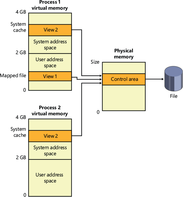
Figure 11-2 Coherent caching scheme.

So, for example, if Process 1 has a view (View 1) of the file mapped into its user address space, and Process 2 is accessing the same view via the system cache, Process 2 sees any changes that Process 1 makes as they’re made, not as they’re flushed. The memory manager won’t flush all user-mapped pages—only those that it knows have been written to (because they have the modified bit set). Therefore, any process accessing a file under Windows always sees the most up-to-date version of that file, even if some processes have the file open through the I/O system and others have the file mapped into their address space using the Windows file mapping functions.

Note

Cache coherency in this case refers to coherency between user-mapped data and cached I/O and not between noncached and cached hardware access and I/Os, which are almost guaranteed to be incoherent. Also, cache coherency is somewhat more difficult for network redirectors than for local file systems because network redirectors must implement additional flushing and purge operations to ensure cache coherency when accessing network data.

Virtual block caching

The Windows cache manager uses a method known as virtual block caching, in which the cache manager keeps track of which parts of which files are in the cache. The cache manager is able to monitor these file portions by mapping 256 KB views of files into system virtual address spaces, using special system cache routines located in the memory manager. This approach has the following key benefits:

• ■    It opens up the possibility of doing intelligent read-ahead; because the cache tracks which parts of which files are in the cache, it can predict where the caller might be going next.

• ■    It allows the I/O system to bypass going to the file system for requests for data that is already in the cache (fast I/O). Because the cache manager knows which parts of which files are in the cache, it can return the address of cached data to satisfy an I/O request without having to call the file system.

Details of how intelligent read-ahead and fast I/O work are provided later in this chapter in the “Fast I/O” and “Read-ahead and write-behind” sections.

Stream-based caching

The cache manager is also designed to do stream caching rather than file caching. A stream is a sequence of bytes within a file. Some file systems, such as NTFS, allow a file to contain more than one stream; the cache manager accommodates such file systems by caching each stream independently. NTFS can exploit this feature by organizing its master file table (described later in this chapter in the “Master file table” section) into streams and by caching these streams as well. In fact, although the cache manager might be said to cache files, it actually caches streams (all files have at least one stream of data) identified by both a file name and, if more than one stream exists in the file, a stream name.

Note

Internally, the cache manager is not aware of file or stream names but uses pointers to these structures.

Recoverable file system support

Recoverable file systems such as NTFS are designed to reconstruct the disk volume structure after a system failure. This capability means that I/O operations in progress at the time of a system failure must be either entirely completed or entirely backed out from the disk when the system is restarted. Half-completed I/O operations can corrupt a disk volume and even render an entire volume inaccessible. To avoid this problem, a recoverable file system maintains a log file in which it records every update it intends to make to the file system structure (the file system’s metadata) before it writes the change to the volume. If the system fails, interrupting volume modifications in progress, the recoverable file system uses information stored in the log to reissue the volume updates.

To guarantee a successful volume recovery, every log file record documenting a volume update must be completely written to disk before the update itself is applied to the volume. Because disk writes are cached, the cache manager and the file system must coordinate metadata updates by ensuring that the log file is flushed ahead of metadata updates. Overall, the following actions occur in sequence:

1. The file system writes a log file record documenting the metadata update it intends to make.

2. The file system calls the cache manager to flush the log file record to disk.

3. The file system writes the volume update to the cache—that is, it modifies its cached metadata.

4. The cache manager flushes the altered metadata to disk, updating the volume structure. (Actually, log file records are batched before being flushed to disk, as are volume modifications.)

Note

The term metadata applies only to changes in the file system structure: file and directory creation, renaming, and deletion.

When a file system writes data to the cache, it can supply a logical sequence number (LSN) that identifies the record in its log file, which corresponds to the cache update. The cache manager keeps track of these numbers, recording the lowest and highest LSNs (representing the oldest and newest log file records) associated with each page in the cache. In addition, data streams that are protected by transaction log records are marked as “no write” by NTFS so that the mapped page writer won’t inadvertently write out these pages before the corresponding log records are written. (When the mapped page writer sees a page marked this way, it moves the page to a special list that the cache manager then flushes at the appropriate time, such as when lazy writer activity takes place.)

When it prepares to flush a group of dirty pages to disk, the cache manager determines the highest LSN associated with the pages to be flushed and reports that number to the file system. The file system can then call the cache manager back, directing it to flush log file data up to the point represented by the reported LSN. After the cache manager flushes the log file up to that LSN, it flushes the corresponding volume structure updates to disk, thus ensuring that it records what it’s going to do before actually doing it. These interactions between the file system and the cache manager guarantee the recoverability of the disk volume after a system failure.

NTFS MFT working set enhancements

As we have described in the previous paragraphs, the mechanism that the cache manager uses to cache files is the same as general memory mapped I/O interfaces provided by the memory manager to the operating system. For accessing or caching a file, the cache manager maps a view of the file in the system virtual address space. The contents are then accessed simply by reading off the mapped virtual address range. When the cached content of a file is no longer needed (for various reasons—see the next paragraphs for details), the cache manager unmaps the view of the file. This strategy works well for any kind of data files but has some problems with the metadata that the file system maintains for correctly storing the files in the volume.

When a file handle is closed (or the owning process dies), the cache manager ensures that the cached data is no longer in the working set. The NTFS file system accesses the Master File Table (MFT) as a big file, which is cached like any other user files by the cache manager. The problem with the MFT is that, since it is a system file, which is mapped and processed in the System process context, nobody will ever close its handle (unless the volume is unmounted), so the system never unmaps any cached view of the MFT. The process that initially caused a particular view of MFT to be mapped might have closed the handle or exited, leaving potentially unwanted views of MFT still mapped into memory consuming valuable system cache (these views will be unmapped only if the system runs into memory pressure).

Windows 8.1 resolved this problem by storing a reference counter to every MFT record in a dynamically allocated multilevel array, which is stored in the NTFS file system Volume Control Block (VCB) structure. Every time a File Control Block (FCB) data structure is created (further details on the FCB and VCB are available later in this chapter), the file system increases the counter of the relative MFT index record. In the same way, when the FCB is destroyed (meaning that all the handles to the file or directory that the MFT entry refers to are closed), NTFS dereferences the relative counter and calls the CcUnmapFileOffsetFromSystemCache cache manager routine, which will unmap the part of the MFT that is no longer needed.

Memory partitions support

Windows 10, with the goal to provide support for Hyper-V containers containers and game mode, introduced the concept of partitions. Memory partitions have already been described in Chapter 5 of Part 1. As seen in that chapter, memory partitions are represented by a large data structure (MI_PARTITION), which maintains memory-related management structures related to the partition, such as page lists (standby, modified, zero, free, and so on), commit charge, working set, page trimmer, modified page writer, and zero-page thread. The cache manager needs to cooperate with the memory manager in order to support partitions. During phase 1 of NT kernel initialization, the system creates and initializes the cache manager partition (for further details about Windows kernel initialization, see Chapter 12, “Startup and shutdown”), which will be part of the System Executive partition (MemoryPartition0). The cache manager’s code has gone through a big refactoring to support partitions; all the global cache manager data structures and variables have been moved in the cache manager partition data structure (CC_PARTITION).

The cache manager’s partition contains cache-related data, like the global shared cache maps list, the worker threads list (read-ahead, write-behind, and extra write-behind; lazy writer and lazy writer scan; async reads), lazy writer scan events, an array that holds the history of write-behind throughout, the upper and lower limit for the dirty pages threshold, the number of dirty pages, and so on. When the cache manager system partition is initialized, all the needed system threads are started in the context of a System process which belongs to the partition. Each partition always has an associated minimal System process, which is created at partition-creation time (by the NtCreatePartition API).

When the system creates a new partition through the NtCreatePartition API, it always creates and initializes an empty MI_PARTITION object (the memory is moved from a parent partition to the child, or hot-added later by using the NtManagePartition function). A cache manager partition object is created only on-demand. If no files are created in the context of the new partition, there is no need to create the cache manager partition object. When the file system creates or opens a file for caching access, the CcinitializeCacheMap(Ex) function checks which partition the file belongs to and whether the partition has a valid link to a cache manager partition. In case there is no cache manager partition, the system creates and initializes a new one through the CcCreatePartition routine. The new partition starts separate cache manager-related threads (read-ahead, lazy writers, and so on) and calculates the new values of the dirty page threshold based on the number of pages that belong to the specific partition.

The file object contains a link to the partition it belongs to through its control area, which is initially allocated by the file system driver when creating and mapping the Stream Control Block (SCB). The partition of the target file is stored into a file object extension (of type MemoryPartitionInformation) and is checked by the memory manager when creating the section object for the SCB. In general, files are shared entities, so there is no way for File System drivers to automatically associate a file to a different partition than the System Partition. An application can set a different partition for a file using the NtSetInformationFileKernel API, through the new FileMemoryPartitionInformation class.

Cache virtual memory management

Because the Windows system cache manager caches data on a virtual basis, it uses up regions of system virtual address space (instead of physical memory) and manages them in structures called virtual address control blocks, or VACBs. VACBs define these regions of address space into 256 KB slots called views. When the cache manager initializes during the bootup process, it allocates an initial array of VACBs to describe cached memory. As caching requirements grow and more memory is required, the cache manager allocates more VACB arrays, as needed. It can also shrink virtual address space as other demands put pressure on the system.

At a file’s first I/O (read or write) operation, the cache manager maps a 256 KB view of the 256 KB-aligned region of the file that contains the requested data into a free slot in the system cache address space. For example, if 10 bytes starting at an offset of 300,000 bytes were read into a file, the view that would be mapped would begin at offset 262144 (the second 256 KB-aligned region of the file) and extend for 256 KB.

The cache manager maps views of files into slots in the cache’s address space on a round-robin basis, mapping the first requested view into the first 256 KB slot, the second view into the second 256 KB slot, and so forth, as shown in Figure 11-3. In this example, File B was mapped first, File A second, and File C third, so File B’s mapped chunk occupies the first slot in the cache. Notice that only the first 256 KB portion of File B has been mapped, which is due to the fact that only part of the file has been accessed. Because File C is only 100 KB (and thus smaller than one of the views in the system cache), it requires its own 256 KB slot in the cache.

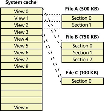
Figure 11-3 Files of varying sizes mapped into the system cache.

The cache manager guarantees that a view is mapped as long as it’s active (although views can remain mapped after they become inactive). A view is marked active, however, only during a read or write operation to or from the file. Unless a process opens a file by specifying the FILE_FLAG_RANDOM_ ACCESS flag in the call to CreateFile, the cache manager unmaps inactive views of a file as it maps new views for the file if it detects that the file is being accessed sequentially. Pages for unmapped views are sent to the standby or modified lists (depending on whether they have been changed), and because the memory manager exports a special interface for the cache manager, the cache manager can direct the pages to be placed at the end or front of these lists. Pages that correspond to views of files opened with the FILE_FLAG_SEQUENTIAL_SCAN flag are moved to the front of the lists, whereas all others are moved to the end. This scheme encourages the reuse of pages belonging to sequentially read files and specifically prevents a large file copy operation from affecting more than a small part of physical memory. The flag also affects unmapping. The cache manager will aggressively unmap views when this flag is supplied.

If the cache manager needs to map a view of a file, and there are no more free slots in the cache, it will unmap the least recently mapped inactive view and use that slot. If no views are available, an I/O error is returned, indicating that insufficient system resources are available to perform the operation. Given that views are marked active only during a read or write operation, however, this scenario is extremely unlikely because thousands of files would have to be accessed simultaneously for this situation to occur.

Cache size

In the following sections, we explain how Windows computes the size of the system cache, both virtually and physically. As with most calculations related to memory management, the size of the system cache depends on a number of factors.

Cache virtual size

On a 32-bit Windows system, the virtual size of the system cache is limited solely by the amount of kernel-mode virtual address space and the SystemCacheLimit registry key that can be optionally configured. (See Chapter 5 of Part 1 for more information on limiting the size of the kernel virtual address space.) This means that the cache size is capped by the 2-GB system address space, but it is typically significantly smaller because the system address space is shared with other resources, including system paged table entries (PTEs), nonpaged and paged pool, and page tables. The maximum virtual cache size is 64 TB on 64-bit Windows, and even in this case, the limit is still tied to the system address space size: in future systems that will support the 56-bit addressing mode, the limit will be 32 PB (petabytes).

Cache working set size

As mentioned earlier, one of the key differences in the design of the cache manager in Windows from that of other operating systems is the delegation of physical memory management to the global memory manager. Because of this, the existing code that handles working set expansion and trimming, as well as managing the modified and standby lists, is also used to control the size of the system cache, dynamically balancing demands for physical memory between processes and the operating system.

The system cache doesn’t have its own working set but shares a single system set that includes cache data, paged pool, pageable kernel code, and pageable driver code. As explained in the section “System working sets” in Chapter 5 of Part 1, this single working set is called internally the system cache working set even though the system cache is just one of the components that contribute to it. For the purposes of this book, we refer to this working set simply as the system working set. Also explained in Chapter 5 is the fact that if the LargeSystemCache registry value is 1, the memory manager favors the system working set over that of processes running on the system.

Cache physical size

While the system working set includes the amount of physical memory that is mapped into views in the cache’s virtual address space, it does not necessarily reflect the total amount of file data that is cached in physical memory. There can be a discrepancy between the two values because additional file data might be in the memory manager’s standby or modified page lists.

Recall from Chapter 5 that during the course of working set trimming or page replacement, the memory manager can move dirty pages from a working set to either the standby list or the modified page list, depending on whether the page contains data that needs to be written to the paging file or another file before the page can be reused. If the memory manager didn’t implement these lists, any time a process accessed data previously removed from its working set, the memory manager would have to hard-fault it in from disk. Instead, if the accessed data is present on either of these lists, the memory manager simply soft-faults the page back into the process’s working set. Thus, the lists serve as in-memory caches of data that are stored in the paging file, executable images, or data files. Thus, the total amount of file data cached on a system includes not only the system working set but the combined sizes of the standby and modified page lists as well.

An example illustrates how the cache manager can cause much more file data than that containable in the system working set to be cached in physical memory. Consider a system that acts as a dedicated file server. A client application accesses file data from across the network, while a server, such as the file server driver (%SystemRoot%\System32\Drivers\Srv2.sys, described later in this chapter), uses cache manager interfaces to read and write file data on behalf of the client. If the client reads through several thousand files of 1 MB each, the cache manager will have to start reusing views when it runs out of mapping space (and can’t enlarge the VACB mapping area). For each file read thereafter, the cache manager unmaps views and remaps them for new files. When the cache manager unmaps a view, the memory manager doesn’t discard the file data in the cache’s working set that corresponds to the view; it moves the data to the standby list. In the absence of any other demand for physical memory, the standby list can consume almost all the physical memory that remains outside the system working set. In other words, virtually all the server’s physical memory will be used to cache file data, as shown in Figure 11-4.

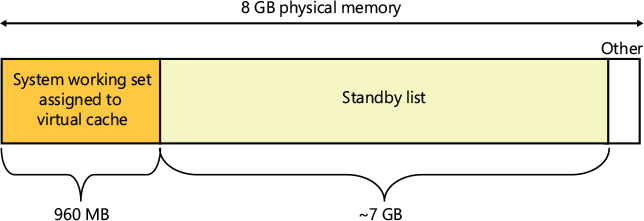
Figure 11-4 Example in which most of physical memory is being used by the file cache.

Because the total amount of file data cached includes the system working set, modified page list, and standby list—the sizes of which are all controlled by the memory manager—it is in a sense the real cache manager. The cache manager subsystem simply provides convenient interfaces for accessing file data through the memory manager. It also plays an important role with its read-ahead and write-behind policies in influencing what data the memory manager keeps present in physical memory, as well as with managing system virtual address views of the space.

To try to accurately reflect the total amount of file data that’s cached on a system, Task Manager shows a value named “Cached” in its performance view that reflects the combined size of the system working set, standby list, and modified page list. Process Explorer, on the other hand, breaks up these values into Cache WS (system cache working set), Standby, and Modified. Figure 11-5 shows the system information view in Process Explorer and the Cache WS value in the Physical Memory area in the lower left of the figure, as well as the size of the standby and modified lists in the Paging Lists area near the middle of the figure. Note that the Cache value in Task Manager also includes the Paged WS, Kernel WS, and Driver WS values shown in Process Explorer. When these values were chosen, the vast majority of System WS came from the Cache WS. This is no longer the case today, but the anachronism remains in Task Manager.

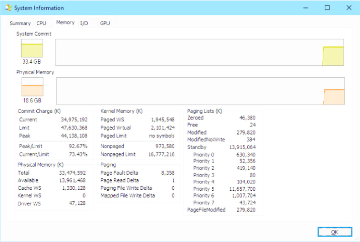
Figure 11-5 Process Explorer’s System Information dialog box.

Cache data structures

The cache manager uses the following data structures to keep track of cached files:

• ■    Each 256 KB slot in the system cache is described by a VACB.

• ■    Each separately opened cached file has a private cache map, which contains information used to control read-ahead (discussed later in the chapter in the “Intelligent read-ahead” section).

• ■    Each cached file has a single shared cache map structure, which points to slots in the system cache that contain mapped views of the file.

These structures and their relationships are described in the next sections.

Systemwide cache data structures

As previously described, the cache manager keeps track of the state of the views in the system cache by using an array of data structures called virtual address control block (VACB) arrays that are stored in nonpaged pool. On a 32-bit system, each VACB is 32 bytes in size and a VACB array is 128 KB, resulting in 4,096 VACBs per array. On a 64-bit system, a VACB is 40 bytes, resulting in 3,276 VACBs per array. The cache manager allocates the initial VACB array during system initialization and links it into the systemwide list of VACB arrays called CcVacbArrays. Each VACB represents one 256 KB view in the system cache, as shown in Figure 11-6. The structure of a VACB is shown in Figure 11-7.

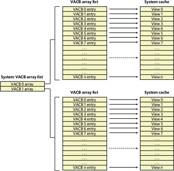
Figure 11-6 System VACB array.

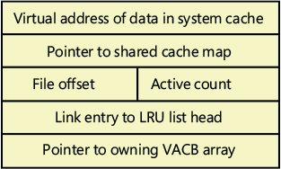
Figure 11-7 VACB data structure.

Additionally, each VACB array is composed of two kinds of VACB: low priority mapping VACBs and high priority mapping VACBs. The system allocates 64 initial high priority VACBs for each VACB array. High priority VACBs have the distinction of having their views preallocated from system address space. When the memory manager has no views to give to the cache manager at the time of mapping some data, and if the mapping request is marked as high priority, the cache manager will use one of the preallocated views present in a high priority VACB. It uses these high priority VACBs, for example, for critical file system metadata as well as for purging data from the cache. After high priority VACBs are gone, however, any operation requiring a VACB view will fail with insufficient resources. Typically, the mapping priority is set to the default of low, but by using the PIN_HIGH_PRIORITY flag when pinning (described later) cached data, file systems can request a high priority VACB to be used instead, if one is needed.

As you can see in Figure 11-7, the first field in a VACB is the virtual address of the data in the system cache. The second field is a pointer to the shared cache map structure, which identifies which file is cached. The third field identifies the offset within the file at which the view begins (always based on 256 KB granularity). Given this granularity, the bottom 16 bits of the file offset will always be zero, so those bits are reused to store the number of references to the view—that is, how many active reads or writes are accessing the view. The fourth field links the VACB into a list of least-recently-used (LRU) VACBs when the cache manager frees the VACB; the cache manager first checks this list when allocating a new VACB. Finally, the fifth field links this VACB to the VACB array header representing the array in which the VACB is stored.

During an I/O operation on a file, the file’s VACB reference count is incremented, and then it’s decremented when the I/O operation is over. When the reference count is nonzero, the VACB is active. For access to file system metadata, the active count represents how many file system drivers have the pages in that view locked into memory.

EXPERIMENT: Looking at VACBs and VACB statistics

The cache manager internally keeps track of various values that are useful to developers and support engineers when debugging crash dumps. All these debugging variables start with the CcDbg prefix, which makes it easy to see the whole list, thanks to the x command:

Click here to view code image

1: kd> x nt!*ccdbg*
    fffff800`d052741c nt!CcDbgNumberOfFailedWorkQueueEntryAllocations = <no type information>
    fffff800`d05276ec nt!CcDbgNumberOfNoopedReadAheads = <no type information>
    fffff800`d05276e8 nt!CcDbgLsnLargerThanHint = <no type information>
    fffff800`d05276e4 nt!CcDbgAdditionalPagesQueuedCount = <no type information>
    fffff800`d0543370 nt!CcDbgFoundAsyncReadThreadListEmpty = <no type information>
    fffff800`d054336c nt!CcDbgNumberOfCcUnmapInactiveViews = <no type information>
    fffff800`d05276e0 nt!CcDbgSkippedReductions = <no type information>
    fffff800`d0542e04 nt!CcDbgDisableDAX = <no type information>
    ...

Some systems may show differences in variable names due to 32-bit versus 64-bit implementations. The exact variable names are irrelevant in this experiment—focus instead on the methodology that is explained. Using these variables and your knowledge of the VACB array header data structures, you can use the kernel debugger to list all the VACB array headers. The CcVacbArrays variable is an array of pointers to VACB array headers, which you dereference to dump the contents of the _VACB_ARRAY_HEADERs. First, obtain the highest array index:

Click here to view code image

1: kd> dd nt!CcVacbArraysHighestUsedIndex  l1
    fffff800`d0529c1c  00000000

And now you can dereference each index until the maximum index. On this system (and this is the norm), the highest index is 0, which means there’s only one header to dereference:

Click here to view code image

1: kd> ?? (*((nt!_VACB_ARRAY_HEADER***)@@(nt!CcVacbArrays)))[0]
    struct _VACB_ARRAY_HEADER * 0xffffc40d`221cb000
       +0x000 VacbArrayIndex   : 0
       +0x004 MappingCount     : 0x302
       +0x008 HighestMappedIndex : 0x301
       +0x00c Reserved         : 0

If there were more, you could change the array index at the end of the command with a higher number, until you reach the highest used index. The output shows that the system has only one VACB array with 770 (0x302) active VACBs.

Finally, the CcNumberOfFreeVacbs variable stores the number of VACBs on the free VACB list. Dumping this variable on the system used for the experiment results in 2,506 (0x9ca):

Click here to view code image

1: kd> dd nt!CcNumberOfFreeVacbs  l1
    fffff800`d0527318  000009ca

As expected, the sum of the free (0x9ca—2,506 decimal) and active VACBs (0x302—770 decimal) on a 64-bit system with one VACB array equals 3,276, the number of VACBs in one VACB array. If the system were to run out of free VACBs, the cache manager would try to allocate a new VACB array. Because of the volatile nature of this experiment, your system may create and/or free additional VACBs between the two steps (dumping the active and then the free VACBs). This might cause your total of free and active VACBs to not match exactly 3,276. Try quickly repeating the experiment a couple of times if this happens, although you may never get stable numbers, especially if there is lots of file system activity on the system.

Per-file cache data structures

Each open handle to a file has a corresponding file object. (File objects are explained in detail in Chapter 6 of Part 1, “I/O system.”) If the file is cached, the file object points to a private cache map structure that contains the location of the last two reads so that the cache manager can perform intelligent read-ahead (described later, in the section “Intelligent read-ahead”). In addition, all the private cache maps for open instances of a file are linked together.

Each cached file (as opposed to file object) has a shared cache map structure that describes the state of the cached file, including the partition to which it belongs, its size, and its valid data length. (The function of the valid data length field is explained in the section “Write-back caching and lazy writing.”) The shared cache map also points to the section object (maintained by the memory manager and which describes the file’s mapping into virtual memory), the list of private cache maps associated with that file, and any VACBs that describe currently mapped views of the file in the system cache. (See Chapter 5 of Part 1 for more about section object pointers.) All the opened shared cache maps for different files are linked in a global linked list maintained in the cache manager’s partition data structure. The relationships among these per-file cache data structures are illustrated in Figure 11-8.

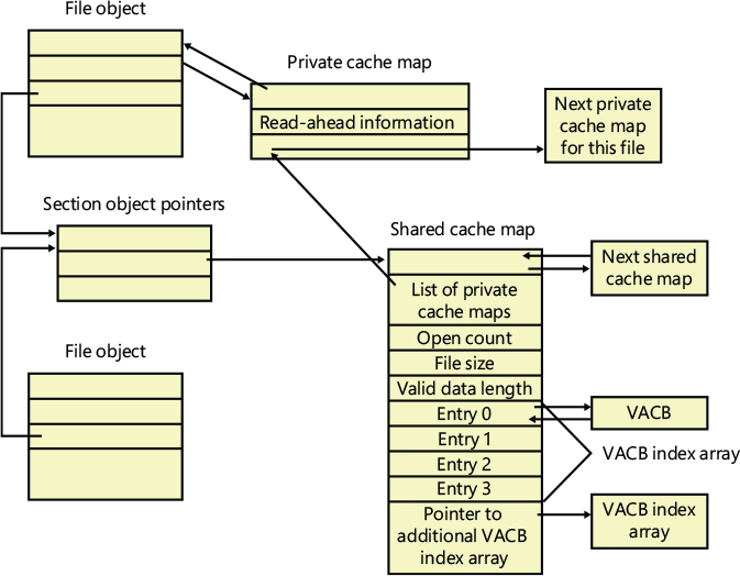
Figure 11-8 Per-file cache data structures.

When asked to read from a particular file, the cache manager must determine the answers to two questions:

1. Is the file in the cache?

2. If so, which VACB, if any, refers to the requested location?

In other words, the cache manager must find out whether a view of the file at the desired address is mapped into the system cache. If no VACB contains the desired file offset, the requested data isn’t currently mapped into the system cache.

To keep track of which views for a given file are mapped into the system cache, the cache manager maintains an array of pointers to VACBs, which is known as the VACB index array. The first entry in the VACB index array refers to the first 256 KB of the file, the second entry to the second 256 KB, and so on. The diagram in Figure 11-9 shows four different sections from three different files that are currently mapped into the system cache.

When a process accesses a particular file in a given location, the cache manager looks in the appropriate entry in the file’s VACB index array to see whether the requested data has been mapped into the cache. If the array entry is nonzero (and hence contains a pointer to a VACB), the area of the file being referenced is in the cache. The VACB, in turn, points to the location in the system cache where the view of the file is mapped. If the entry is zero, the cache manager must find a free slot in the system cache (and therefore a free VACB) to map the required view.

As a size optimization, the shared cache map contains a VACB index array that is four entries in size. Because each VACB describes 256 KB, the entries in this small, fixed-size index array can point to VACB array entries that together describe a file of up to 1 MB. If a file is larger than 1 MB, a separate VACB index array is allocated from nonpaged pool, based on the size of the file divided by 256 KB and rounded up in the case of a remainder. The shared cache map then points to this separate structure.

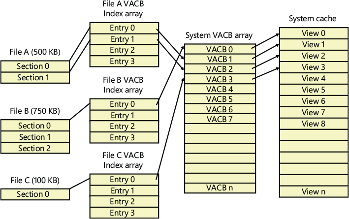
Figure 11-9 VACB index arrays.

As a further optimization, the VACB index array allocated from nonpaged pool becomes a sparse multilevel index array if the file is larger than 32 MB, where each index array consists of 128 entries. You can calculate the number of levels required for a file with the following formula:

(Number of bits required to represent file size – 18) / 7

Round up the result of the equation to the next whole number. The value 18 in the equation comes from the fact that a VACB represents 256 KB, and 256 KB is 2^18. The value 7 comes from the fact that each level in the array has 128 entries and 2^7 is 128. Thus, a file that has a size that is the maximum that can be described with 63 bits (the largest size the cache manager supports) would require only seven levels. The array is sparse because the only branches that the cache manager allocates are ones for which there are active views at the lowest-level index array. Figure 11-10 shows an example of a multilevel VACB array for a sparse file that is large enough to require three levels.

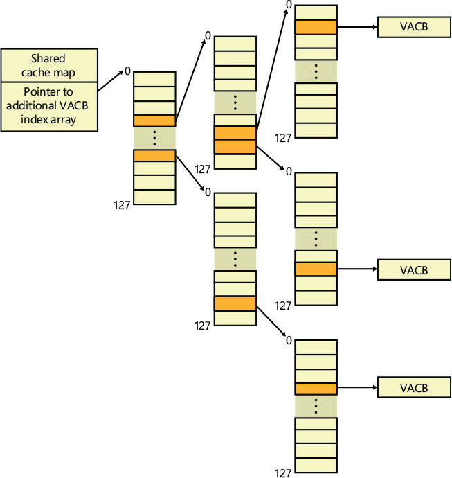
Figure 11-10 Multilevel VACB arrays.

This scheme is required to efficiently handle sparse files that might have extremely large file sizes with only a small fraction of valid data because only enough of the array is allocated to handle the currently mapped views of a file. For example, a 32-GB sparse file for which only 256 KB is mapped into the cache’s virtual address space would require a VACB array with three allocated index arrays because only one branch of the array has a mapping and a 32-GB file requires a three-level array. If the cache manager didn’t use the multilevel VACB index array optimization for this file, it would have to allocate a VACB index array with 128,000 entries, or the equivalent of 1,000 VACB index arrays.

File system interfaces

The first time a file’s data is accessed for a cached read or write operation, the file system driver is responsible for determining whether some part of the file is mapped in the system cache. If it’s not, the file system driver must call the CcInitializeCacheMap function to set up the per-file data structures described in the preceding section.

Once a file is set up for cached access, the file system driver calls one of several functions to access the data in the file. There are three primary methods for accessing cached data, each intended for a specific situation:

• ■    The copy method copies user data between cache buffers in system space and a process buffer in user space.

• ■    The mapping and pinning method uses virtual addresses to read and write data directly from and to cache buffers.

• ■    The physical memory access method uses physical addresses to read and write data directly from and to cache buffers.

File system drivers must provide two versions of the file read operation—cached and noncached—to prevent an infinite loop when the memory manager processes a page fault. When the memory manager resolves a page fault by calling the file system to retrieve data from the file (via the device driver, of course), it must specify this as a paging read operation by setting the “no cache” and “paging IO” flags in the IRP.

Figure 11-11 illustrates the typical interactions between the cache manager, the memory manager, and file system drivers in response to user read or write file I/O. The cache manager is invoked by a file system through the copy interfaces (the CcCopyRead and CcCopyWrite paths). To process a CcFastCopyRead or CcCopyRead read, for example, the cache manager creates a view in the cache to map a portion of the file being read and reads the file data into the user buffer by copying from the view. The copy operation generates page faults as it accesses each previously invalid page in the view, and in response the memory manager initiates noncached I/O into the file system driver to retrieve the data corresponding to the part of the file mapped to the page that faulted.

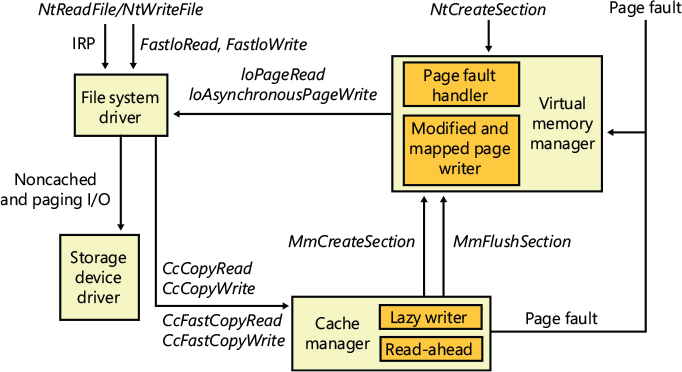
Figure 11-11 File system interaction with cache and memory managers.

The next three sections explain these cache access mechanisms, their purpose, and how they’re used.

Copying to and from the cache

Because the system cache is in system space, it’s mapped into the address space of every process. As with all system space pages, however, cache pages aren’t accessible from user mode because that would be a potential security hole. (For example, a process might not have the rights to read a file whose data is currently contained in some part of the system cache.) Thus, user application file reads and writes to cached files must be serviced by kernel-mode routines that copy data between the cache’s buffers in system space and the application’s buffers residing in the process address space.

Caching with the mapping and pinning interfaces

Just as user applications read and write data in files on a disk, file system drivers need to read and write the data that describes the files themselves (the metadata, or volume structure data). Because the file system drivers run in kernel mode, however, they could, if the cache manager were properly informed, modify data directly in the system cache. To permit this optimization, the cache manager provides functions that permit the file system drivers to find where in virtual memory the file system metadata resides, thus allowing direct modification without the use of intermediary buffers.

If a file system driver needs to read file system metadata in the cache, it calls the cache manager’s mapping interface to obtain the virtual address of the desired data. The cache manager touches all the requested pages to bring them into memory and then returns control to the file system driver. The file system driver can then access the data directly.

If the file system driver needs to modify cache pages, it calls the cache manager’s pinning services, which keep the pages active in virtual memory so that they can’t be reclaimed. The pages aren’t actually locked into memory (such as when a device driver locks pages for direct memory access transfers). Most of the time, a file system driver will mark its metadata stream as no write, which instructs the memory manager’s mapped page writer (explained in Chapter 5 of Part 1) to not write the pages to disk until explicitly told to do so. When the file system driver unpins (releases) them, the cache manager releases its resources so that it can lazily flush any changes to disk and release the cache view that the metadata occupied.

The mapping and pinning interfaces solve one thorny problem of implementing a file system: buffer management. Without directly manipulating cached metadata, a file system must predict the maximum number of buffers it will need when updating a volume’s structure. By allowing the file system to access and update its metadata directly in the cache, the cache manager eliminates the need for buffers, simply updating the volume structure in the virtual memory the memory manager provides. The only limitation the file system encounters is the amount of available memory.

Caching with the direct memory access interfaces

In addition to the mapping and pinning interfaces used to access metadata directly in the cache, the cache manager provides a third interface to cached data: direct memory access (DMA). The DMA functions are used to read from or write to cache pages without intervening buffers, such as when a network file system is doing a transfer over the network.

The DMA interface returns to the file system the physical addresses of cached user data (rather than the virtual addresses, which the mapping and pinning interfaces return), which can then be used to transfer data directly from physical memory to a network device. Although small amounts of data (1 KB to 2 KB) can use the usual buffer-based copying interfaces, for larger transfers the DMA interface can result in significant performance improvements for a network server processing file requests from remote systems. To describe these references to physical memory, a memory descriptor list (MDL) is used. (MDLs are introduced in Chapter 5 of Part 1.)

Fast I/O

Whenever possible, reads and writes to cached files are handled by a high-speed mechanism named fast I/O. Fast I/O is a means of reading or writing a cached file without going through the work of generating an IRP. With fast I/O, the I/O manager calls the file system driver’s fast I/O routine to see whether I/O can be satisfied directly from the cache manager without generating an IRP.

Because the cache manager is architected on top of the virtual memory subsystem, file system drivers can use the cache manager to access file data simply by copying to or from pages mapped to the actual file being referenced without going through the overhead of generating an IRP.

Fast I/O doesn’t always occur. For example, the first read or write to a file requires setting up the file for caching (mapping the file into the cache and setting up the cache data structures, as explained earlier in the section “Cache data structures”). Also, if the caller specified an asynchronous read or write, fast I/O isn’t used because the caller might be stalled during paging I/O operations required to satisfy the buffer copy to or from the system cache and thus not really providing the requested asynchronous I/O operation. But even on a synchronous I/O operation, the file system driver might decide that it can’t process the I/O operation by using the fast I/O mechanism—say, for example, if the file in question has a locked range of bytes (as a result of calls to the Windows LockFile and UnlockFile functions). Because the cache manager doesn’t know what parts of which files are locked, the file system driver must check the validity of the read or write, which requires generating an IRP. The decision tree for fast I/O is shown in Figure 11-12.

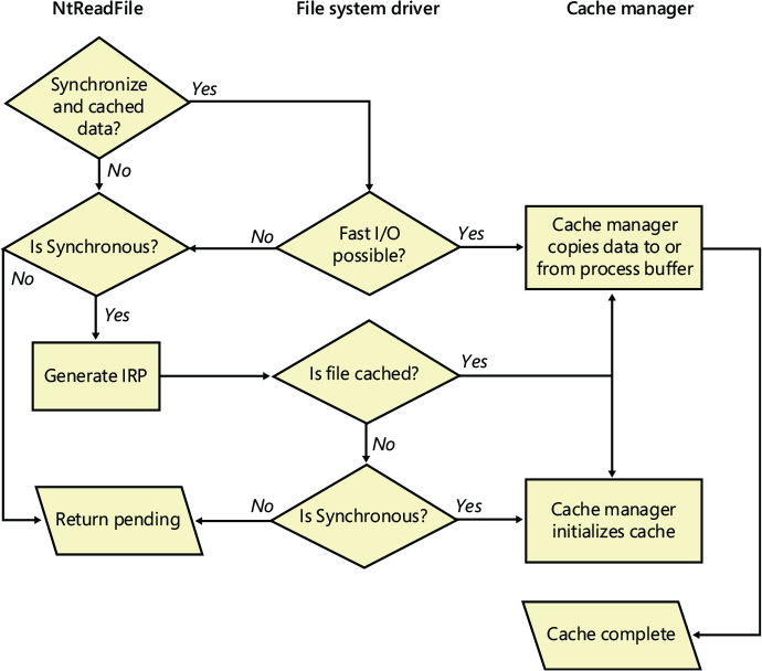
Figure 11-12 Fast I/O decision tree.

These steps are involved in servicing a read or a write with fast I/O:

1. A thread performs a read or write operation.

2. If the file is cached and the I/O is synchronous, the request passes to the fast I/O entry point of the file system driver stack. If the file isn’t cached, the file system driver sets up the file for caching so that the next time, fast I/O can be used to satisfy a read or write request.

3. If the file system driver’s fast I/O routine determines that fast I/O is possible, it calls the cache manager’s read or write routine to access the file data directly in the cache. (If fast I/O isn’t possible, the file system driver returns to the I/O system, which then generates an IRP for the I/O and eventually calls the file system’s regular read routine.)

4. The cache manager translates the supplied file offset into a virtual address in the cache.

5. For reads, the cache manager copies the data from the cache into the buffer of the process requesting it; for writes, it copies the data from the buffer to the cache.

6. One of the following actions occurs:

   • •    For reads where FILE_FLAG_RANDOM_ACCESS wasn’t specified when the file was opened, the read-ahead information in the caller’s private cache map is updated. Read-ahead may also be queued for files for which the FO_RANDOM_ACCESS flag is not specified.

   • •    For writes, the dirty bit of any modified page in the cache is set so that the lazy writer will know to flush it to disk.

   • •    For write-through files, any modifications are flushed to disk.

Read-ahead and write-behind

In this section, you’ll see how the cache manager implements reading and writing file data on behalf of file system drivers. Keep in mind that the cache manager is involved in file I/O only when a file is opened without the FILE_FLAG_NO_BUFFERING flag and then read from or written to using the Windows I/O functions (for example, using the Windows ReadFile and WriteFile functions). Mapped files don’t go through the cache manager, nor do files opened with the FILE_FLAG_NO_BUFFERING flag set.

Note

When an application uses the FILE_FLAG_NO_BUFFERING flag to open a file, its file I/O must start at device-aligned offsets and be of sizes that are a multiple of the alignment size; its input and output buffers must also be device-aligned virtual addresses. For file systems, this usually corresponds to the sector size (4,096 bytes on NTFS, typically, and 2,048 bytes on CDFS). One of the benefits of the cache manager, apart from the actual caching performance, is the fact that it performs intermediate buffering to allow arbitrarily aligned and sized I/O.

Intelligent read-ahead

The cache manager uses the principle of spatial locality to perform intelligent read-ahead by predicting what data the calling process is likely to read next based on the data that it’s reading currently. Because the system cache is based on virtual addresses, which are contiguous for a particular file, it doesn’t matter whether they’re juxtaposed in physical memory. File read-ahead for logical block caching is more complex and requires tight cooperation between file system drivers and the block cache because that cache system is based on the relative positions of the accessed data on the disk, and, of course, files aren’t necessarily stored contiguously on disk. You can examine read-ahead activity by using the Cache: Read Aheads/sec performance counter or the CcReadAheadIos system variable.

Reading the next block of a file that is being accessed sequentially provides an obvious performance improvement, with the disadvantage that it will cause head seeks. To extend read-ahead benefits to cases of stridden data accesses (both forward and backward through a file), the cache manager maintains a history of the last two read requests in the private cache map for the file handle being accessed, a method known as asynchronous read-ahead with history. If a pattern can be determined from the caller’s apparently random reads, the cache manager extrapolates it. For example, if the caller reads page 4,000 and then page 3,000, the cache manager assumes that the next page the caller will require is page 2,000 and prereads it.

Note

Although a caller must issue a minimum of three read operations to establish a predictable sequence, only two are stored in the private cache map.

To make read-ahead even more efficient, the Win32 CreateFile function provides a flag indicating forward sequential file access: FILE_FLAG_SEQUENTIAL_SCAN. If this flag is set, the cache manager doesn’t keep a read history for the caller for prediction but instead performs sequential read-ahead. However, as the file is read into the cache’s working set, the cache manager unmaps views of the file that are no longer active and, if they are unmodified, directs the memory manager to place the pages belonging to the unmapped views at the front of the standby list so that they will be quickly reused. It also reads ahead two times as much data (2 MB instead of 1 MB, for example). As the caller continues reading, the cache manager prereads additional blocks of data, always staying about one read (of the size of the current read) ahead of the caller.

The cache manager’s read-ahead is asynchronous because it’s performed in a thread separate from the caller’s thread and proceeds concurrently with the caller’s execution. When called to retrieve cached data, the cache manager first accesses the requested virtual page to satisfy the request and then queues an additional I/O request to retrieve additional data to a system worker thread. The worker thread then executes in the background, reading additional data in anticipation of the caller’s next read request. The preread pages are faulted into memory while the program continues executing so that when the caller requests the data it’s already in memory.

For applications that have no predictable read pattern, the FILE_FLAG_RANDOM_ACCESS flag can be specified when the CreateFile function is called. This flag instructs the cache manager not to attempt to predict where the application is reading next and thus disables read-ahead. The flag also stops the cache manager from aggressively unmapping views of the file as the file is accessed so as to minimize the mapping/unmapping activity for the file when the application revisits portions of the file.

Read-ahead enhancements

Windows 8.1 introduced some enhancements to the cache manager read-ahead functionality. File system drivers and network redirectors can decide the size and growth for the intelligent read-ahead with the CcSetReadAheadGranularityEx API function. The cache manager client can decide the following:

• ■    Read-ahead granularity Sets the minimum read-ahead unit size and the end file-offset of the next read-ahead. The cache manager sets the default granularity to 4 Kbytes (the size of a memory page), but every file system sets this value in a different way (NTFS, for example, sets the cache granularity to 64 Kbytes).

  Figure 11-13 shows an example of read-ahead on a 200 Kbyte-sized file, where the cache granularity has been set to 64 KB. If the user requests a nonaligned 1 KB read at offset 0x10800, and if a sequential read has already been detected, the intelligent read-ahead will emit an I/O that encompasses the 64 KB of data from offset 0x10000 to 0x20000. If there were already more than two sequential reads, the cache manager emits another supplementary read from offset 0x20000 to offset 0x30000 (192 Kbytes).

  

  Figure 11-13 Read-ahead on a 200 KB file, with granularity set to 64KB.

• ■    Pipeline size For some remote file system drivers, it may make sense to split large read-ahead I/Os into smaller chunks, which will be emitted in parallel by the cache manager worker threads. A network file system can achieve a substantial better throughput using this technique.

• ■    Read-ahead aggressiveness File system drivers can specify the percentage used by the cache manager to decide how to increase the read-ahead size after the detection of a third sequential read. For example, let’s assume that an application is reading a big file using a 1 Mbyte I/O size. After the tenth read, the application has already read 10 Mbytes (the cache manager may have already prefetched some of them). The intelligent read-ahead now decides by how much to grow the read-ahead I/O size. If the file system has specified 60% of growth, the formula used is the following:

  (Number of sequential reads * Size of last read) * (Growth percentage / 100)

  So, this means that the next read-ahead size is 6 MB (instead of being 2 MB, assuming that the granularity is 64 KB and the I/O size is 1 MB). The default growth percentage is 50% if not modified by any cache manager client.

Write-back caching and lazy writing

The cache manager implements a write-back cache with lazy write. This means that data written to files is first stored in memory in cache pages and then written to disk later. Thus, write operations are allowed to accumulate for a short time and are then flushed to disk all at once, reducing the overall number of disk I/O operations.

The cache manager must explicitly call the memory manager to flush cache pages because otherwise the memory manager writes memory contents to disk only when demand for physical memory exceeds supply, as is appropriate for volatile data. Cached file data, however, represents nonvolatile disk data. If a process modifies cached data, the user expects the contents to be reflected on disk in a timely manner.

Additionally, the cache manager has the ability to veto the memory manager’s mapped writer thread. Since the modified list (see Chapter 5 of Part 1 for more information) is not sorted in logical block address (LBA) order, the cache manager’s attempts to cluster pages for larger sequential I/Os to the disk are not always successful and actually cause repeated seeks. To combat this effect, the cache manager has the ability to aggressively veto the mapped writer thread and stream out writes in virtual byte offset (VBO) order, which is much closer to the LBA order on disk. Since the cache manager now owns these writes, it can also apply its own scheduling and throttling algorithms to prefer read-ahead over write-behind and impact the system less.

The decision about how often to flush the cache is an important one. If the cache is flushed too frequently, system performance will be slowed by unnecessary I/O. If the cache is flushed too rarely, you risk losing modified file data in the cases of a system failure (a loss especially irritating to users who know that they asked the application to save the changes) and running out of physical memory (because it’s being used by an excess of modified pages).

To balance these concerns, the cache manager’s lazy writer scan function executes on a system worker thread once per second. The lazy writer scan has different duties:

• ■    Checks the number of average available pages and dirty pages (that belongs to the current partition) and updates the dirty page threshold’s bottom and the top limits accordingly. The threshold itself is updated too, primarily based on the total number of dirty pages written in the previous cycle (see the following paragraphs for further details). It sleeps if there are no dirty pages to write.

• ■    Calculates the number of dirty pages to write to disk through the CcCalculatePagesToWrite internal routine. If the number of dirty pages is more than 256 (1 MB of data), the cache manager queues one-eighth of the total dirty pages to be flushed to disk. If the rate at which dirty pages are being produced is greater than the amount the lazy writer had determined it should write, the lazy writer writes an additional number of dirty pages that it calculates are necessary to match that rate.

• ■    Cycles between each shared cache map (which are stored in a linked list belonging to the current partition), and, using the internal CcShouldLazyWriteCacheMap routine, determines if the current file described by the shared cache map needs to be flushed to disk. There are different reasons why a file shouldn’t be flushed to disk: for example, an I/O could have been already initialized by another thread, the file could be a temporary file, or, more simply, the cache map might not have any dirty pages. In case the routine determined that the file should be flushed out, the lazy writer scan checks whether there are still enough available pages to write, and, if so, posts a work item to the cache manager system worker threads.

Note

The lazy writer scan uses some exceptions while deciding the number of dirty pages mapped by a particular shared cache map to write (it doesn’t always write all the dirty pages of a file): If the target file is a metadata stream with more than 256 KB of dirty pages, the cache manager writes only one-eighth of its total pages. Another exception is used for files that have more dirty pages than the total number of pages that the lazy writer scan can flush.

Lazy writer system worker threads from the systemwide critical worker thread pool actually perform the I/O operations. The lazy writer is also aware of when the memory manager’s mapped page writer is already performing a flush. In these cases, it delays its write-back capabilities to the same stream to avoid a situation where two flushers are writing to the same file.

Note

The cache manager provides a means for file system drivers to track when and how much data has been written to a file. After the lazy writer flushes dirty pages to the disk, the cache manager notifies the file system, instructing it to update its view of the valid data length for the file. (The cache manager and file systems separately track in memory the valid data length for a file.)

EXPERIMENT: Watching the cache manager in action

In this experiment, we use Process Monitor to view the underlying file system activity, including cache manager read-ahead and write-behind, when Windows Explorer copies a large file (in this example, a DVD image) from one local directory to another.

First, configure Process Monitor’s filter to include the source and destination file paths, the Explorer.exe and System processes, and the ReadFile and WriteFile operations. In this example, the C:\Users\Andrea\Documents\Windows_10_RS3.iso file was copied to C:\ISOs\ Windows_10_RS3.iso, so the filter is configured as follows:

You should see a Process Monitor trace like the one shown here after you copy the file:

The first few entries show the initial I/O processing performed by the copy engine and the first cache manager operations. Here are some of the things that you can see:

• ■    The initial 1 MB cached read from Explorer at the first entry. The size of this read depends on an internal matrix calculation based on the file size and can vary from 128 KB to 1 MB. Because this file was large, the copy engine chose 1 MB.

• ■    The 1-MB read is followed by another 1-MB noncached read. Noncached reads typically indicate activity due to page faults or cache manager access. A closer look at the stack trace for these events, which you can see by double-clicking an entry and choosing the Stack tab, reveals that indeed the CcCopyRead cache manager routine, which is called by the NTFS driver’s read routine, causes the memory manager to fault the source data into physical memory:

  

• ■    After this 1-MB page fault I/O, the cache manager’s read-ahead mechanism starts reading the file, which includes the System process’s subsequent noncached 1-MB read at the 1-MB offset. Because of the file size and Explorer’s read I/O sizes, the cache manager chose 1 MB as the optimal read-ahead size. The stack trace for one of the read-ahead operations, shown next, confirms that one of the cache manager’s worker threads is performing the read-ahead.

  

After this point, Explorer’s 1-MB reads aren’t followed by page faults, because the read-ahead thread stays ahead of Explorer, prefetching the file data with its 1-MB noncached reads. However, every once in a while, the read-ahead thread is not able to pick up enough data in time, and clustered page faults do occur, which appear as Synchronous Paging I/O.

If you look at the stack for these entries, you’ll see that instead of MmPrefetchForCacheManager, the MmAccessFault/MiIssueHardFault routines are called.

As soon as it starts reading, Explorer also starts performing writes to the destination file. These are sequential, cached 1-MB writes. After about 124 MB of reads, the first WriteFile operation from the System process occurs, shown here:

The write operation’s stack trace, shown here, indicates that the memory manager’s mapped page writer thread was actually responsible for the write. This occurs because for the first couple of megabytes of data, the cache manager hadn’t started performing write-behind, so the memory manager’s mapped page writer began flushing the modified destination file data. (See Chapter 10 for more information on the mapped page writer.)

To get a clearer view of the cache manager operations, remove Explorer from the Process Monitor’s filter so that only the System process operations are visible, as shown next.

With this view, it’s much easier to see the cache manager’s 1-MB write-behind operations (the maximum write sizes are 1 MB on client versions of Windows and 32 MB on server versions; this experiment was performed on a client system). The stack trace for one of the write-behind operations, shown here, verifies that a cache manager worker thread is performing write-behind:

As an added experiment, try repeating this process with a remote copy instead (from one Windows system to another) and by copying files of varying sizes. You’ll notice some different behaviors by the copy engine and the cache manager, both on the receiving and sending sides.

Disabling lazy writing for a file

If you create a temporary file by specifying the flag FILE_ATTRIBUTE_TEMPORARY in a call to the Windows CreateFile function, the lazy writer won’t write dirty pages to the disk unless there is a severe shortage of physical memory or the file is explicitly flushed. This characteristic of the lazy writer improves system performance—the lazy writer doesn’t immediately write data to a disk that might ultimately be discarded. Applications usually delete temporary files soon after closing them.

Forcing the cache to write through to disk

Because some applications can’t tolerate even momentary delays between writing a file and seeing the updates on disk, the cache manager also supports write-through caching on a per-file object basis; changes are written to disk as soon as they’re made. To turn on write-through caching, set the FILE_FLAG_WRITE_THROUGH flag in the call to the CreateFile function. Alternatively, a thread can explicitly flush an open file by using the Windows FlushFileBuffers function when it reaches a point at which the data needs to be written to disk.

Flushing mapped files

If the lazy writer must write data to disk from a view that’s also mapped into another process’s address space, the situation becomes a little more complicated because the cache manager will only know about the pages it has modified. (Pages modified by another process are known only to that process because the modified bit in the page table entries for modified pages is kept in the process private page tables.) To address this situation, the memory manager informs the cache manager when a user maps a file. When such a file is flushed in the cache (for example, as a result of a call to the Windows FlushFileBuffers function), the cache manager writes the dirty pages in the cache and then checks to see whether the file is also mapped by another process. When the cache manager sees that the file is also mapped by another process, the cache manager then flushes the entire view of the section to write out pages that the second process might have modified. If a user maps a view of a file that is also open in the cache, when the view is unmapped, the modified pages are marked as dirty so that when the lazy writer thread later flushes the view, those dirty pages will be written to disk. This procedure works as long as the sequence occurs in the following order:

1. A user unmaps the view.

2. A process flushes file buffers.

If this sequence isn’t followed, you can’t predict which pages will be written to disk.

EXPERIMENT: Watching cache flushes

You can see the cache manager map views into the system cache and flush pages to disk by running the Performance Monitor and adding the Data Maps/sec and Lazy Write Flushes/sec counters. (You can find these counters under the “Cache” group.) Then, copy a large file from one location to another. The generally higher line in the following screenshot shows Data Maps/sec, and the other shows Lazy Write Flushes/sec. During the file copy, Lazy Write Flushes/sec significantly increased.

Write throttling

The file system and cache manager must determine whether a cached write request will affect system performance and then schedule any delayed writes. First, the file system asks the cache manager whether a certain number of bytes can be written right now without hurting performance by using the CcCanIWrite function and blocking that write if necessary. For asynchronous I/O, the file system sets up a callback with the cache manager for automatically writing the bytes when writes are again permitted by calling CcDeferWrite. Otherwise, it just blocks and waits on CcCanIWrite to continue. Once it’s notified of an impending write operation, the cache manager determines how many dirty pages are in the cache and how much physical memory is available. If few physical pages are free, the cache manager momentarily blocks the file system thread that’s requesting to write data to the cache. The cache manager’s lazy writer flushes some of the dirty pages to disk and then allows the blocked file system thread to continue. This write throttling prevents system performance from degrading because of a lack of memory when a file system or network server issues a large write operation.

Note

The effects of write throttling are volume-aware, such that if a user is copying a large file on, say, a RAID-0 SSD while also transferring a document to a portable USB thumb drive, writes to the USB disk will not cause write throttling to occur on the SSD transfer.

The dirty page threshold is the number of pages that the system cache will allow to be dirty before throttling cached writers. This value is computed when the cache manager partition is initialized (the system partition is created and initialized at phase 1 of the NT kernel startup) and depends on the product type (client or server). As seen in the previous paragraphs, two other values are also computed—the top dirty page threshold and the bottom dirty page threshold. Depending on memory consumption and the rate at which dirty pages are being processed, the lazy writer scan calls the internal function CcAdjustThrottle, which, on server systems, performs dynamic adjustment of the current threshold based on the calculated top and bottom values. This adjustment is made to preserve the read cache in cases of a heavy write load that will inevitably overrun the cache and become throttled. Table 11-1 lists the algorithms used to calculate the dirty page thresholds.

Table 11-1 Algorithms for calculating the dirty page thresholds

Product Type	Dirty Page Threshold	Top Dirty Page Threshold	Bottom Dirty Page Threshold
Client	Physical pages / 8	Physical pages / 8	Physical pages / 8
Server	Physical pages / 2	Physical pages / 2	Physical pages / 8

Write throttling is also useful for network redirectors transmitting data over slow communication lines. For example, suppose a local process writes a large amount of data to a remote file system over a slow 640 Kbps line. The data isn’t written to the remote disk until the cache manager’s lazy writer flushes the cache. If the redirector has accumulated lots of dirty pages that are flushed to disk at once, the recipient could receive a network timeout before the data transfer completes. By using the CcSetDirtyPageThreshold function, the cache manager allows network redirectors to set a limit on the number of dirty cache pages they can tolerate (for each stream), thus preventing this scenario. By limiting the number of dirty pages, the redirector ensures that a cache flush operation won’t cause a network timeout.

System threads

As mentioned earlier, the cache manager performs lazy write and read-ahead I/O operations by submitting requests to the common critical system worker thread pool. However, it does limit the use of these threads to one less than the total number of critical system worker threads. In client systems, there are 5 total critical system worker threads, whereas in server systems there are 10.

Internally, the cache manager organizes its work requests into four lists (though these are serviced by the same set of executive worker threads):

• ■    The express queue is used for read-ahead operations.

• ■    The regular queue is used for lazy write scans (for dirty data to flush), write-behinds, and lazy closes.

• ■    The fast teardown queue is used when the memory manager is waiting for the data section owned by the cache manager to be freed so that the file can be opened with an image section instead, which causes CcWriteBehind to flush the entire file and tear down the shared cache map.

• ■    The post tick queue is used for the cache manager to internally register for a notification after each “tick” of the lazy writer thread—in other words, at the end of each pass.

To keep track of the work items the worker threads need to perform, the cache manager creates its own internal per-processor look-aside list—a fixed-length list (one for each processor) of worker queue item structures. (Look-aside lists are discussed in Chapter 5 of Part 1.) The number of worker queue items depends on system type: 128 for client systems, and 256 for server systems. For cross-processor performance, the cache manager also allocates a global look-aside list at the same sizes as just described.

Aggressive write behind and low-priority lazy writes

With the goal of improving cache manager performance, and to achieve compatibility with low-speed disk devices (like eMMC disks), the cache manager lazy writer has gone through substantial improvements in Windows 8.1 and later.

As seen in the previous paragraphs, the lazy writer scan adjusts the dirty page threshold and its top and bottom limits. Multiple adjustments are made on the limits, by analyzing the history of the total number of available pages. Other adjustments are performed to the dirty page threshold itself by checking whether the lazy writer has been able to write the expected total number of pages in the last execution cycle (one per second). If the total number of written pages in the last cycle is less than the expected number (calculated by the CcCalculatePagesToWrite routine), it means that the underlying disk device was not able to support the generated I/O throughput, so the dirty page threshold is lowered (this means that more I/O throttling is performed, and some cache manager clients will wait when calling CcCanIWrite API). In the opposite case, in which there are no remaining pages from the last cycle, the lazy writer scan can easily raise the threshold. In both cases, the threshold needs to stay inside the range described by the bottom and top limits.

The biggest improvement has been made thanks to the Extra Write Behind worker threads. In server SKUs, the maximum number of these threads is nine (which corresponds to the total number of critical system worker threads minus one), while in client editions it is only one. When a system lazy write scan is requested by the cache manager, the system checks whether dirty pages are contributing to memory pressure (using a simple formula that verifies that the number of dirty pages are less than a quarter of the dirty page threshold, and less than half of the available pages). If so, the systemwide cache manager thread pool routine (CcWorkerThread) uses a complex algorithm that determines whether it can add another lazy writer thread that will write dirty pages to disk in parallel with the others.

To correctly understand whether it is possible to add another thread that will emit additional I/Os, without getting worse system performance, the cache manager calculates the disk throughput of the old lazy write cycles and keeps track of their performance. If the throughput of the current cycles is equal or better than the previous one, it means that the disk can support the overall I/O level, so it makes sense to add another lazy writer thread (which is called an Extra Write Behind thread in this case). If, on the other hand, the current throughput is lower than the previous cycle, it means that the underlying disk is not able to sustain additional parallel writes, so the Extra Write Behind thread is removed. This feature is called Aggressive Write Behind.

In Windows client editions, the cache manager enables an optimization designed to deal with low-speed disks. When a lazy writer scan is requested, and when the file system drivers write to the cache, the cache manager employs an algorithm to decide if the lazy writers threads should execute at low priority. (For more information about thread priorities, refer to Chapter 4 of Part 1.) The cache manager applies by-default low priority to the lazy writers if the following conditions are met (otherwise, the cache manager still uses the normal priority):

• ■    The caller is not waiting for the current lazy scan to be finished.

• ■    The total size of the partition’s dirty pages is less than 32 MB.

If the two conditions are satisfied, the cache manager queues the work items for the lazy writers in the low-priority queue. The lazy writers are started by a system worker thread, which executes at priority 6 – Lowest. Furthermore, the lazy writer set its I/O priority to Lowest just before emitting the actual I/O to the correct file-system driver.

Dynamic memory

As seen in the previous paragraph, the dirty page threshold is calculated dynamically based on the available amount of physical memory. The cache manager uses the threshold to decide when to throttle incoming writes and whether to be more aggressive about writing behind.

Before the introduction of partitions, the calculation was made in the CcInitializeCacheManager routine (by checking the MmNumberOfPhysicalPages global value), which was executed during the kernel’s phase 1 initialization. Now, the cache manager Partition’s initialization function performs the calculation based on the available physical memory pages that belong to the associated memory partition. (For further details about cache manager partitions, see the section “Memory partitions support,” earlier in this chapter.) This is not enough, though, because Windows also supports the hot-addition of physical memory, a feature that is deeply used by HyperV for supporting dynamic memory for child VMs.

During memory manager phase 0 initialization, MiCreatePfnDatabase calculates the maximum possible size of the PFN database. On 64-bit systems, the memory manager assumes that the maximum possible amount of installed physical memory is equal to all the addressable virtual memory range (256 TB on non-LA57 systems, for example). The system asks the memory manager to reserve the amount of virtual address space needed to store a PFN for each virtual page in the entire address space. (The size of this hypothetical PFN database is around 64 GB.) MiCreateSparsePfnDatabase then cycles between each valid physical memory range that Winload has detected and maps valid PFNs into the database. The PFN database uses sparse memory. When the MiAddPhysicalMemory routines detect new physical memory, it creates new PFNs simply by allocating new regions inside the PFN databases. Dynamic Memory has already been described in Chapter 9, “Virtualization technologies”; further details are available there.

The cache manager needs to detect the new hot-added or hot-removed memory and adapt to the new system configuration, otherwise multiple problems could arise:

• ■    In cases where new memory has been hot-added, the cache manager might think that the system has less memory, so its dirty pages threshold is lower than it should be. As a result, the cache manager doesn’t cache as many dirty pages as it should, so it throttles writes much sooner.

• ■    If large portions of available memory are locked or aren’t available anymore, performing cached I/O on the system could hurt the responsiveness of other applications (which, after the hot-remove, will basically have no more memory).

To correctly deal with this situation, the cache manager doesn’t register a callback with the memory manager but implements an adaptive correction in the lazy writer scan (LWS) thread. Other than scanning the list of shared cache map and deciding which dirty page to write, the LWS thread has the ability to change the dirty pages threshold depending on foreground rate, its write rate, and available memory. The LWS maintains a history of average available physical pages and dirty pages that belong to the partition. Every second, the LWS thread updates these lists and calculates aggregate values. Using the aggregate values, the LWS is able to respond to memory size variations, absorbing the spikes and gradually modifying the top and bottom thresholds.

Cache manager disk I/O accounting

Before Windows 8.1, it wasn’t possible to precisely determine the total amount of I/O performed by a single process. The reasons behind this were multiple:

• ■    Lazy writes and read-aheads don’t happen in the context of the process/thread that caused the I/O. The cache manager writes out the data lazily, completing the write in a different context (usually the System context) of the thread that originally wrote the file. (The actual I/O can even happen after the process has terminated.) Likewise, the cache manager can choose to read-ahead, bringing in more data from the file than the process requested.

• ■    Asynchronous I/O is still managed by the cache manager, but there are cases in which the cache manager is not involved at all, like for non-cached I/Os.

• ■    Some specialized applications can emit low-level disk I/O using a lower-level driver in the disk stack.

Windows stores a pointer to the thread that emitted the I/O in the tail of the IRP. This thread is not always the one that originally started the I/O request. As a result, a lot of times the I/O accounting was wrongly associated with the System process. Windows 8.1 resolved the problem by introducing the PsUpdateDiskCounters API, used by both the cache manager and file system drivers, which need to tightly cooperate. The function stores the total number of bytes read and written and the number of I/O operations in the core EPROCESS data structure that is used by the NT kernel to describe a process. (You can read more details in Chapter 3 of Part 1.)

The cache manager updates the process disk counters (by calling the PsUpdateDiskCounters function) while performing cached reads and writes (through all of its exposed file system interfaces) and while emitting read-aheads I/O (through CcScheduleReadAheadEx exported API). NTFS and ReFS file systems drivers call the PsUpdateDiskCounters while performing non-cached and paging I/O.

Like CcScheduleReadAheadEx, multiple cache manager APIs have been extended to accept a pointer to the thread that has emitted the I/O and should be charged for it (CcCopyReadEx and CcCopyWriteEx are good examples). In this way, updated file system drivers can even control which thread to charge in case of asynchronous I/O.

Other than per-process counters, the cache manager also maintains a Global Disk I/O counter, which globally keeps track of all the I/O that has been issued by file systems to the storage stack. (The counter is updated every time a non-cached and paging I/O is emitted through file system drivers.) Thus, this global counter, when subtracted from the total I/O emitted to a particular disk device (a value that an application can obtain by using the IOCTL_DISK_PERFORMANCE control code), represents the I/O that could not be attributed to any particular process (paging I/O emitted by the Modified Page Writer for example, or I/O performed internally by Mini-filter drivers).

The new per-process disk counters are exposed through the NtQuerySystemInformation API using the SystemProcessInformation information class. This is the method that diagnostics tools like Task Manager or Process Explorer use for precisely querying the I/O numbers related to the processes currently running in the system.

EXPERIMENT: Counting disk I/Os

You can see a precise counting of the total system I/Os by using the different counters exposed by the Performance Monitor. Open Performance Monitor and add the FileSystem Bytes Read and FileSystem Bytes Written counters, which are available in the FileSystem Disk Activity group. Furthermore, for this experiment you need to add the per-process disk I/O counters that are available in the Process group, named IO Read Bytes/sec and IO Write Bytes/sec. When you add these last two counters, make sure that you select the Explorer process in the Instances Of Selected Object box.

When you start to copy a big file, you see the counters belonging to Explorer processes increasing until they reach the counters showed in the global file System Disk activity.

File systems

In this section, we present an overview of the supported file system formats supported by Windows. We then describe the types of file system drivers and their basic operation, including how they interact with other system components, such as the memory manager and the cache manager. Following that, we describe in detail the functionality and the data structures of the two most important file systems: NTFS and ReFS. We start by analyzing their internal architectures and then focus on the on-disk layout of the two file systems and their advanced features, such as compression, recoverability, encryption, tiering support, file-snapshot, and so on.

Windows file system formats

Windows includes support for the following file system formats:

• ■    CDFS

• ■    UDF

• ■    FAT12, FAT16, and FAT32

• ■    exFAT

• ■    NTFS

• ■    ReFS

Each of these formats is best suited for certain environments, as you’ll see in the following sections.

CDFS

CDFS (%SystemRoot%\System32\Drivers\Cdfs.sys), or CD-ROM file system, is a read-only file system driver that supports a superset of the ISO-9660 format as well as a superset of the Joliet disk format. Although the ISO-9660 format is relatively simple and has limitations such as ASCII uppercase names with a maximum length of 32 characters, Joliet is more flexible and supports Unicode names of arbitrary length. If structures for both formats are present on a disk (to offer maximum compatibility), CDFS uses the Joliet format. CDFS has a couple of restrictions:

• ■    A maximum file size of 4 GB

• ■    A maximum of 65,535 directories

CDFS is considered a legacy format because the industry has adopted the Universal Disk Format (UDF) as the standard for optical media.

UDF

The Windows Universal Disk Format (UDF) file system implementation is OSTA (Optical Storage Technology Association) UDF-compliant. (UDF is a subset of the ISO-13346 format with extensions for formats such as CD-R and DVD-R/RW.) OSTA defined UDF in 1995 as a format to replace the ISO-9660 format for magneto-optical storage media, mainly DVD-ROM. UDF is included in the DVD specification and is more flexible than CDFS. The UDF file system format has the following traits:

• ■    Directory and file names can be 254 ASCII or 127 Unicode characters long.

• ■    Files can be sparse. (Sparse files are defined later in this chapter, in the “Compression and sparse files” section.)

• ■    File sizes are specified with 64 bits.

• ■    Support for access control lists (ACLs).

• ■    Support for alternate data streams.

The UDF driver supports UDF versions up to 2.60. The UDF format was designed with rewritable media in mind. The Windows UDF driver (%SystemRoot%\System32\Drivers\Udfs.sys) provides read-write support for Blu-ray, DVD-RAM, CD-R/RW, and DVD+-R/RW drives when using UDF 2.50 and read-only support when using UDF 2.60. However, Windows does not implement support for certain UDF features such as named streams and access control lists.

FAT12, FAT16, and FAT32

Windows supports the FAT file system primarily for compatibility with other operating systems in multiboot systems, and as a format for flash drives or memory cards. The Windows FAT file system driver is implemented in %SystemRoot%\System32\Drivers\Fastfat.sys.

The name of each FAT format includes a number that indicates the number of bits that the particular format uses to identify clusters on a disk. FAT12’s 12-bit cluster identifier limits a partition to storing a maximum of 2¹² (4,096) clusters. Windows permits cluster sizes from 512 bytes to 8 KB, which limits a FAT12 volume size to 32 MB.

Note

All FAT file system types reserve the first 2 clusters and the last 16 clusters of a volume, so the number of usable clusters for a FAT12 volume, for instance, is slightly less than 4,096.

FAT16, with a 16-bit cluster identifier, can address 2¹⁶ (65,536) clusters. On Windows, FAT16 cluster sizes range from 512 bytes (the sector size) to 64 KB (on disks with a 512-byte sector size), which limits FAT16 volume sizes to 4 GB. Disks with a sector size of 4,096 bytes allow for clusters of 256 KB. The cluster size Windows uses depends on the size of a volume. The various sizes are listed in Table 11-2. If you format a volume that is less than 16 MB as FAT by using the format command or the Disk Management snap-in, Windows uses the FAT12 format instead of FAT16.

Table 11-2 Default FAT16 cluster sizes in Windows

Volume Size	Default Cluster Size
<8 MB	Not supported
8 MB–32 MB	512 bytes
32 MB–64 MB	1 KB
64 MB–128 MB	2 KB
128 MB–256 MB	4 KB
256 MB–512 MB	8 KB
512 MB–1,024 MB	16 KB
1 GB–2 GB	32 KB
2 GB–4 GB	64 KB
>16 GB	Not supported

A FAT volume is divided into several regions, which are shown in Figure 11-14. The file allocation table, which gives the FAT file system format its name, has one entry for each cluster on a volume. Because the file allocation table is critical to the successful interpretation of a volume’s contents, the FAT format maintains two copies of the table so that if a file system driver or consistency-checking program (such as Chkdsk) can’t access one (because of a bad disk sector, for example), it can read from the other.

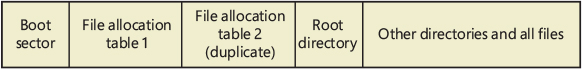
Figure 11-14 FAT format organization.

Entries in the file allocation table define file-allocation chains (shown in Figure 11-15) for files and directories, where the links in the chain are indexes to the next cluster of a file’s data. A file’s directory entry stores the starting cluster of the file. The last entry of the file’s allocation chain is the reserved value of 0xFFFF for FAT16 and 0xFFF for FAT12. The FAT entries for unused clusters have a value of 0. You can see in Figure 11-15 that FILE1 is assigned clusters 2, 3, and 4; FILE2 is fragmented and uses clusters 5, 6, and 8; and FILE3 uses only cluster 7. Reading a file from a FAT volume can involve reading large portions of a file allocation table to traverse the file’s allocation chains.

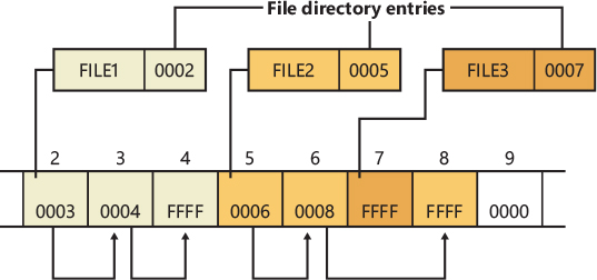
Figure 11-15 Sample FAT file-allocation chains.

The root directory of FAT12 and FAT16 volumes is preassigned enough space at the start of a volume to store 256 directory entries, which places an upper limit on the number of files and directories that can be stored in the root directory. (There’s no preassigned space or size limit on FAT32 root directories.) A FAT directory entry is 32 bytes and stores a file’s name, size, starting cluster, and time stamp (last-accessed, created, and so on) information. If a file has a name that is Unicode or that doesn’t follow the MS-DOS 8.3 naming convention, additional directory entries are allocated to store the long file name. The supplementary entries precede the file’s main entry. Figure 11-16 shows a sample directory entry for a file named “The quick brown fox.” The system has created a THEQUI~1.FOX 8.3 representation of the name (that is, you don’t see a “.” in the directory entry because it is assumed to come after the eighth character) and used two more directory entries to store the Unicode long file name. Each row in the figure is made up of 16 bytes.

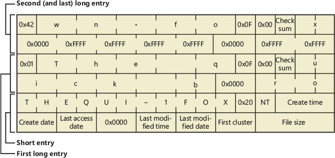
Figure 11-16 FAT directory entry.

FAT32 uses 32-bit cluster identifiers but reserves the high 4 bits, so in effect it has 28-bit cluster identifiers. Because FAT32 cluster sizes can be as large as 64 KB, FAT32 has a theoretical ability to address 16-terabyte (TB) volumes. Although Windows works with existing FAT32 volumes of larger sizes (created in other operating systems), it limits new FAT32 volumes to a maximum of 32 GB. FAT32’s higher potential cluster numbers let it manage disks more efficiently than FAT16; it can handle up to 128-GB volumes with 512-byte clusters. Table 11-3 shows default cluster sizes for FAT32 volumes.

Table 11-3 Default cluster sizes for FAT32 volumes

Partition Size	Default Cluster Size
<32 MB	Not supported
32 MB–64 MB	512 bytes
64 MB–128 MB	1 KB
128 MB–256 MB	2 KB
256 MB–8 GB	4 KB
8 GB–16 GB	8 KB
16 GB–32 GB	16 KB
>32 GB	Not supported

Besides the higher limit on cluster numbers, other advantages FAT32 has over FAT12 and FAT16 include the fact that the FAT32 root directory isn’t stored at a predefined location on the volume, the root directory doesn’t have an upper limit on its size, and FAT32 stores a second copy of the boot sector for reliability. A limitation FAT32 shares with FAT16 is that the maximum file size is 4 GB because directories store file sizes as 32-bit values.

exFAT

Designed by Microsoft, the Extended File Allocation Table file system (exFAT, also called FAT64) is an improvement over the traditional FAT file systems and is specifically designed for flash drives. The main goal of exFAT is to provide some of the advanced functionality offered by NTFS without the metadata structure overhead and metadata logging that create write patterns not suited for many flash media devices. Table 11-4 lists the default cluster sizes for exFAT.

As the FAT64 name implies, the file size limit is increased to 2⁶⁴, allowing files up to 16 exabytes. This change is also matched by an increase in the maximum cluster size, which is currently implemented as 32 MB but can be as large as 2²⁵⁵ sectors. exFAT also adds a bitmap that tracks free clusters, which improves the performance of allocation and deletion operations. Finally, exFAT allows more than 1,000 files in a single directory. These characteristics result in increased scalability and support for large disk sizes.

Table 11-4 Default cluster sizes for exFAT volumes, 512-byte sector

Volume Size	Default Cluster Size
< 256 MB	4 KB
256 MB–32 GB	32 KB
32 GB–512 GB	128 KB
512 GB–1 TB	256 KB
1 TB–2 TB	512 KB
2 TB–4 TB	1 MB
4 TB–8 TB	2 MB
8 TB–16 TB	4 MB
16 TB–32 TB	8 MB
32 TB–64 TB	16 MB
>= 64 TB	32 MB

Additionally, exFAT implements certain features previously available only in NTFS, such as support for access control lists (ACLs) and transactions (called Transaction-Safe FAT, or TFAT). While the Windows Embedded CE implementation of exFAT includes these features, the version of exFAT in Windows does not.

Note

ReadyBoost (described in Chapter 5 of Part 1, “Memory Management”) can work with exFAT-formatted flash drives to support cache files much larger than 4 GB.

NTFS

As noted at the beginning of the chapter, the NTFS file system is one of the native file system formats of Windows. NTFS uses 64-bit cluster numbers. This capacity gives NTFS the ability to address volumes of up to 16 exaclusters; however, Windows limits the size of an NTFS volume to that addressable with 32-bit clusters, which is slightly less than 8 petabytes (using 2 MB clusters). Table 11-5 shows the default cluster sizes for NTFS volumes. (You can override the default when you format an NTFS volume.) NTFS also supports 2³²–1 files per volume. The NTFS format allows for files that are 16 exabytes in size, but the implementation limits the maximum file size to 16 TB.

Table 11-5 Default cluster sizes for NTFS volumes

Volume Size	Default Cluster Size
<7 MB	Not supported
7 MB–16 TB	4 KB
16 TB–32 TB	8 KB
32 TB–64 TB	16 KB
64 TB–128 TB	32 KB
128 TB–256 TB	64 KB
256 TB–512 TB	128 KB
512 TB–1024 TB	256 KB
1 PB–2 PB	512 KB
2 PB–4 PB	1 MB
4 PB–8 PB	2 MB

NTFS includes a number of advanced features, such as file and directory security, alternate data streams, disk quotas, sparse files, file compression, symbolic (soft) and hard links, support for transactional semantics, junction points, and encryption. One of its most significant features is recoverability. If a system is halted unexpectedly, the metadata of a FAT volume can be left in an inconsistent state, leading to the corruption of large amounts of file and directory data. NTFS logs changes to metadata in a transactional manner so that file system structures can be repaired to a consistent state with no loss of file or directory structure information. (File data can be lost unless the user is using TxF, which is covered later in this chapter.) Additionally, the NTFS driver in Windows also implements self-healing, a mechanism through which it makes most minor repairs to corruption of file system on-disk structures while Windows is running and without requiring a reboot.

Note

At the time of this writing, the common physical sector size of disk devices is 4 KB. Even for these disk devices, for compatibility reasons, the storage stack exposes to file system drivers a logical sector size of 512 bytes. The calculation performed by the NTFS driver to determine the correct size of the cluster uses logical sector sizes rather than the actual physical size.

Starting with Windows 10, NTFS supports DAX volumes natively. (DAX volumes are discussed later in this chapter, in the “DAX volumes” section.) The NTFS file system driver also supports I/O to this kind of volume using large pages. Mapping a file that resides on a DAX volume using large pages is possible in two ways: NTFS can automatically align the file to a 2-MB cluster boundary, or the volume can be formatted using a 2-MB cluster size.

ReFS

The Resilient File System (ReFS) is another file system that Windows supports natively. It has been designed primarily for large storage servers with the goal to overcome some limitations of NTFS, like its lack of online self-healing or volume repair or the nonsupport for file snapshots. ReFS is a “write-to-new” file system, which means that volume metadata is always updated by writing new data to the underlying medium and by marking the old metadata as deleted. The lower level of the ReFS file system (which understands the on-disk data structure) uses an object store library, called Minstore, that provides a key-value table interface to its callers. Minstore is similar to a modern database engine, is portable, and uses different data structures and algorithms compared to NTFS. (Minstore uses B+ trees.)

One of the important design goals of ReFS was to be able to support huge volumes (that could have been created by Storage Spaces). Like NTFS, ReFS uses 64-bit cluster numbers and can address volumes of up 16 exaclusters. ReFS has no limitation on the size of the addressable values, so, theoretically, ReFS is able to manage volumes of up to 1 yottabyte (using 64 KB cluster sizes).

Unlike NTFS, Minstore doesn’t need a central location to store its own metadata on the volume (although the object table could be considered somewhat centralized) and has no limitations on addressable values, so there is no need to support many different sized clusters. ReFS supports only 4 KB and 64 KB cluster sizes. ReFS, at the time of this writing, does not support DAX volumes.

We describe NTFS and ReFS data structures and their advanced features in detail later in this chapter.

File system driver architecture

File system drivers (FSDs) manage file system formats. Although FSDs run in kernel mode, they differ in a number of ways from standard kernel-mode drivers. Perhaps most significant, they must register as an FSD with the I/O manager, and they interact more extensively with the memory manager. For enhanced performance, file system drivers also usually rely on the services of the cache manager. Thus, they use a superset of the exported Ntoskrnl.exe functions that standard drivers use. Just as for standard kernel-mode drivers, you must have the Windows Driver Kit (WDK) to build file system drivers. (See Chapter 1, “Concepts and Tools,” in Part 1 and http://www.microsoft.com/whdc/devtools/wdk for more information on the WDK.)

Windows has two different types of FSDs:

• ■    Local FSDs manage volumes directly connected to the computer.

• ■    Network FSDs allow users to access data volumes connected to remote computers.

Local FSDs

Local FSDs include Ntfs.sys, Refs.sys, Refsv1.sys, Fastfat.sys, Exfat.sys, Udfs.sys, Cdfs.sys, and the RAW FSD (integrated in Ntoskrnl.exe). Figure 11-17 shows a simplified view of how local FSDs interact with the I/O manager and storage device drivers. A local FSD is responsible for registering with the I/O manager. Once the FSD is registered, the I/O manager can call on it to perform volume recognition when applications or the system initially access the volumes. Volume recognition involves an examination of a volume’s boot sector and often, as a consistency check, the file system metadata. If none of the registered file systems recognizes the volume, the system assigns the RAW file system driver to the volume and then displays a dialog box to the user asking if the volume should be formatted. If the user chooses not to format the volume, the RAW file system driver provides access to the volume, but only at the sector level—in other words, the user can only read or write complete sectors.

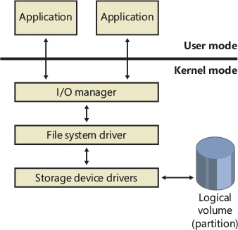
Figure 11-17 Local FSD.

The goal of file system recognition is to allow the system to have an additional option for a valid but unrecognized file system other than RAW. To achieve this, the system defines a fixed data structure type (FILE_SYSTEM_RECOGNITION_STRUCTURE) that is written to the first sector on the volume. This data structure, if present, would be recognized by the operating system, which would then notify the user that the volume contains a valid but unrecognized file system. The system will still load the RAW file system on the volume, but it will not prompt the user to format the volume. A user application or kernel-mode driver might ask for a copy of the FILE_SYSTEM_RECOGNITION_STRUCTURE by using the new file system I/O control code FSCTL_QUERY_FILE_SYSTEM_RECOGNITION.

The first sector of every Windows-supported file system format is reserved as the volume’s boot sector. A boot sector contains enough information so that a local FSD can both identify the volume on which the sector resides as containing a format that the FSD manages and locate any other metadata necessary to identify where metadata is stored on the volume.

When a local FSD (shown in Figure 11-17) recognizes a volume, it creates a device object that represents the mounted file system format. The I/O manager makes a connection through the volume parameter block (VPB) between the volume’s device object (which is created by a storage device driver) and the device object that the FSD created. The VPB’s connection results in the I/O manager redirecting I/O requests targeted at the volume device object to the FSD device object.

To improve performance, local FSDs usually use the cache manager to cache file system data, including metadata. FSDs also integrate with the memory manager so that mapped files are implemented correctly. For example, FSDs must query the memory manager whenever an application attempts to truncate a file to verify that no processes have mapped the part of the file beyond the truncation point. (See Chapter 5 of Part 1 for more information on the memory manager.) Windows doesn’t permit file data that is mapped by an application to be deleted either through truncation or file deletion.

Local FSDs also support file system dismount operations, which permit the system to disconnect the FSD from the volume object. A dismount occurs whenever an application requires raw access to the on-disk contents of a volume or the media associated with a volume is changed. The first time an application accesses the media after a dismount, the I/O manager reinitiates a volume mount operation for the media.

Remote FSDs

Each remote FSD consists of two components: a client and a server. A client-side remote FSD allows applications to access remote files and directories. The client FSD component accepts I/O requests from applications and translates them into network file system protocol commands (such as SMB) that the FSD sends across the network to a server-side component, which is a remote FSD. A server-side FSD listens for commands coming from a network connection and fulfills them by issuing I/O requests to the local FSD that manages the volume on which the file or directory that the command is intended for resides.

Windows includes a client-side remote FSD named LANMan Redirector (usually referred to as just the redirector) and a server-side remote FSD named LANMan Server (%SystemRoot%\System32\Drivers\Srv2.sys). Figure 11-18 shows the relationship between a client accessing files remotely from a server through the redirector and server FSDs.

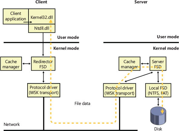
Figure 11-18 Common Internet File System file sharing.

Windows relies on the Common Internet File System (CIFS) protocol to format messages exchanged between the redirector and the server. CIFS is a version of Microsoft’s Server Message Block (SMB) protocol. (For more information on SMB, go to https://docs.microsoft.com/en-us/windows/win32/fileio/microsoft-smb-protocol-and-cifs-protocol-overview.)

Like local FSDs, client-side remote FSDs usually use cache manager services to locally cache file data belonging to remote files and directories, and in such cases both must implement a distributed locking mechanism on the client as well as the server. SMB client-side remote FSDs implement a distributed cache coherency protocol, called oplock (opportunistic locking), so that the data an application sees when it accesses a remote file is the same as the data applications running on other computers that are accessing the same file see. Third-party file systems may choose to use the oplock protocol, or they may implement their own protocol. Although server-side remote FSDs participate in maintaining cache coherency across their clients, they don’t cache data from the local FSDs because local FSDs cache their own data.

It is fundamental that whenever a resource can be shared between multiple, simultaneous accessors, a serialization mechanism must be provided to arbitrate writes to that resource to ensure that only one accessor is writing to the resource at any given time. Without this mechanism, the resource may be corrupted. The locking mechanisms used by all file servers implementing the SMB protocol are the oplock and the lease. Which mechanism is used depends on the capabilities of both the server and the client, with the lease being the preferred mechanism.

Oplocks

The oplock functionality is implemented in the file system run-time library (FsRtlXxx functions) and may be used by any file system driver. The client of a remote file server uses an oplock to dynamically determine which client-side caching strategy to use to minimize network traffic. An oplock is requested on a file residing on a share, by the file system driver or redirector, on behalf of an application when it attempts to open a file. The granting of an oplock allows the client to cache the file rather than send every read or write to the file server across the network. For example, a client could open a file for exclusive access, allowing the client to cache all reads and writes to the file, and then copy the updates to the file server when the file is closed. In contrast, if the server does not grant an oplock to a client, all reads and writes must be sent to the server.

Once an oplock has been granted, a client may then start caching the file, with the type of oplock determining what type of caching is allowed. An oplock is not necessarily held until a client is finished with the file, and it may be broken at any time if the server receives an operation that is incompatible with the existing granted locks. This implies that the client must be able to quickly react to the break of the oplock and change its caching strategy dynamically.

Prior to SMB 2.1, there were four types of oplocks:

• ■    Level 1, exclusive access This lock allows a client to open a file for exclusive access. The client may perform read-ahead buffering and read or write caching.

• ■    Level 2, shared access This lock allows multiple, simultaneous readers of a file and no writers. The client may perform read-ahead buffering and read caching of file data and attributes. A write to the file will cause the holders of the lock to be notified that the lock has been broken.

• ■    Batch, exclusive access This lock takes its name from the locking used when processing batch (.bat) files, which are opened and closed to process each line within the file. The client may keep a file open on the server, even though the application has (perhaps temporarily) closed the file. This lock supports read, write, and handle caching.

• ■    Filter, exclusive access This lock provides applications and file system filters with a mechanism to give up the lock when other clients try to access the same file, but unlike a Level 2 lock, the file cannot be opened for delete access, and the other client will not receive a sharing violation. This lock supports read and write caching.

In the simplest terms, if multiple client systems are all caching the same file shared by a server, then as long as every application accessing the file (from any client or the server) tries only to read the file, those reads can be satisfied from each system’s local cache. This drastically reduces the network traffic because the contents of the file aren’t sent to each system from the server. Locking information must still be exchanged between the client systems and the server, but this requires very low network bandwidth. However, if even one of the clients opens the file for read and write access (or exclusive write), then none of the clients can use their local caches and all I/O to the file must go immediately to the server, even if the file is never written. (Lock modes are based upon how the file is opened, not individual I/O requests.)

An example, shown in Figure 11-19, will help illustrate oplock operation. The server automatically grants a Level 1 oplock to the first client to open a server file for access. The redirector on the client caches the file data for both reads and writes in the file cache of the client machine. If a second client opens the file, it too requests a Level 1 oplock. However, because there are now two clients accessing the same file, the server must take steps to present a consistent view of the file’s data to both clients. If the first client has written to the file, as is the case in Figure 11-19, the server revokes its oplock and grants neither client an oplock. When the first client’s oplock is revoked, or broken, the client flushes any data it has cached for the file back to the server.

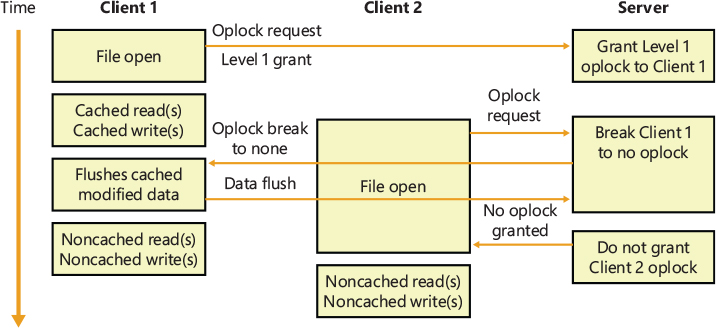
Figure 11-19 Oplock example.

If the first client hadn’t written to the file, the first client’s oplock would have been broken to a Level 2 oplock, which is the same type of oplock the server would grant to the second client. Now both clients can cache reads, but if either writes to the file, the server revokes their oplocks so that noncached operation commences. Once oplocks are broken, they aren’t granted again for the same open instance of a file. However, if a client closes a file and then reopens it, the server reassesses what level of oplock to grant the client based on which other clients have the file open and whether at least one of them has written to the file.

EXPERIMENT: Viewing the list of registered file systems

When the I/O manager loads a device driver into memory, it typically names the driver object it creates to represent the driver so that it’s placed in the \Driver object manager directory. The driver objects for any driver the I/O manager loads that have a Type attribute value of SERVICE_FILE_SYSTEM_DRIVER (2) are placed in the \FileSystem directory by the I/O manager. Thus, using a tool such as WinObj (from Sysinternals), you can see the file systems that have registered on a system, as shown in the following screenshot. Note that file system filter drivers will also show up in this list. Filter drivers are described later in this section.

Another way to see registered file systems is to run the System Information viewer. Run Msinfo32 from the Start menu’s Run dialog box and select System Drivers under Software Environment. Sort the list of drivers by clicking the Type column, and drivers with a Type attribute of SERVICE_FILE_SYSTEM_DRIVER group together.

Note that just because a driver registers as a file system driver type doesn’t mean that it is a local or remote FSD. For example, Npfs (Named Pipe File System) is a driver that implements named pipes through a file system-like private namespace. As mentioned previously, this list will also include file system filter drivers.

Leases

Prior to SMB 2.1, the SMB protocol assumed an error-free network connection between the client and the server and did not tolerate network disconnections caused by transient network failures, server reboot, or cluster failovers. When a network disconnect event was received by the client, it orphaned all handles opened to the affected server(s), and all subsequent I/O operations on the orphaned handles were failed. Similarly, the server would release all opened handles and resources associated with the disconnected user session. This behavior resulted in applications losing state and in unnecessary network traffic.

In SMB 2.1, the concept of a lease is introduced as a new type of client caching mechanism, similar to an oplock. The purpose of a lease and an oplock is the same, but a lease provides greater flexibility and much better performance.

• ■    Read (R), shared access Allows multiple simultaneous readers of a file, and no writers. This lease allows the client to perform read-ahead buffering and read caching.

• ■    Read-Handle (RH), shared access This is similar to the Level 2 oplock, with the added benefit of allowing the client to keep a file open on the server even though the accessor on the client has closed the file. (The cache manager will lazily flush the unwritten data and purge the unmodified cache pages based on memory availability.) This is superior to a Level 2 oplock because the lease does not need to be broken between opens and closes of the file handle. (In this respect, it provides semantics similar to the Batch oplock.) This type of lease is especially useful for files that are repeatedly opened and closed because the cache is not invalidated when the file is closed and refilled when the file is opened again, providing a big improvement in performance for complex I/O intensive applications.

• ■    Read-Write (RW), exclusive access This lease allows a client to open a file for exclusive access. This lock allows the client to perform read-ahead buffering and read or write caching.

• ■    Read-Write-Handle (RWH), exclusive access This lock allows a client to open a file for exclusive access. This lease supports read, write, and handle caching (similar to the Read-Handle lease).

Another advantage that a lease has over an oplock is that a file may be cached, even when there are multiple handles opened to the file on the client. (This is a common behavior in many applications.) This is implemented through the use of a lease key (implemented using a GUID), which is created by the client and associated with the File Control Block (FCB) for the cached file, allowing all handles to the same file to share the same lease state, which provides caching by file rather than caching by handle. Prior to the introduction of the lease, the oplock was broken whenever a new handle was opened to the file, even from the same client. Figure 11-20 shows the oplock behavior, and Figure 11-21 shows the new lease behavior.

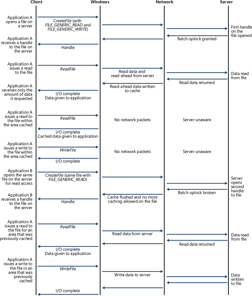
Figure 11-20 Oplock with multiple handles from the same client.

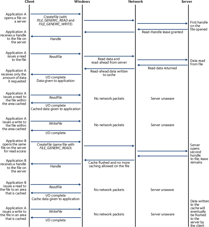
Figure 11-21 Lease with multiple handles from the same client.

Prior to SMB 2.1, oplocks could only be granted or broken, but leases can also be converted. For example, a Read lease may be converted to a Read-Write lease, which greatly reduces network traffic because the cache for a particular file does not need to be invalidated and refilled, as would be the case with an oplock break (of the Level 2 oplock), followed by the request and grant of a Level 1 oplock.

File system operations

Applications and the system access files in two ways: directly, via file I/O functions (such as ReadFile and WriteFile), and indirectly, by reading or writing a portion of their address space that represents a mapped file section. (See Chapter 5 of Part 1 for more information on mapped files.) Figure 11-22 is a simplified diagram that shows the components involved in these file system operations and the ways in which they interact. As you can see, an FSD can be invoked through several paths:

• ■    From a user or system thread performing explicit file I/O

• ■    From the memory manager’s modified and mapped page writers

• ■    Indirectly from the cache manager’s lazy writer

• ■    Indirectly from the cache manager’s read-ahead thread

• ■    From the memory manager’s page fault handler

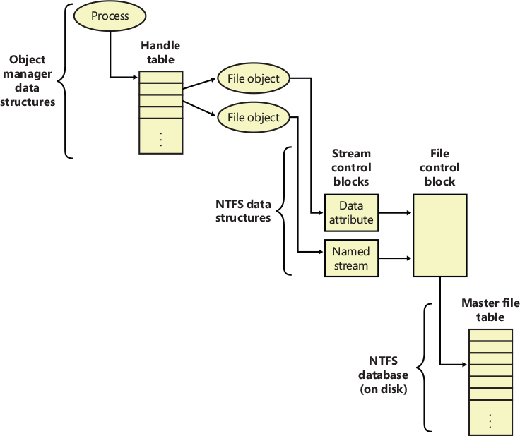
Figure 11-22 Components involved in file system I/O.

The following sections describe the circumstances surrounding each of these scenarios and the steps FSDs typically take in response to each one. You’ll see how much FSDs rely on the memory manager and the cache manager.

Explicit file I/O

The most obvious way an application accesses files is by calling Windows I/O functions such as CreateFile, ReadFile, and WriteFile. An application opens a file with CreateFile and then reads, writes, or deletes the file by passing the handle returned from CreateFile to other Windows functions. The CreateFile function, which is implemented in the Kernel32.dll Windows client-side DLL, invokes the native function NtCreateFile, forming a complete root-relative path name for the path that the application passed to it (processing “.” and “..” symbols in the path name) and prefixing the path with “\??” (for example, \??\C:\Daryl\Todo.txt).

The NtCreateFile system service uses ObOpenObjectByName to open the file, which parses the name starting with the object manager root directory and the first component of the path name (“??”). Chapter 8, “System mechanisms”, includes a thorough description of object manager name resolution and its use of process device maps, but we’ll review the steps it follows here with a focus on volume drive letter lookup.

The first step the object manager takes is to translate \?? to the process’s per-session namespace directory that the DosDevicesDirectory field of the device map structure in the process object references (which was propagated from the first process in the logon session by using the logon session references field in the logon session’s token). Only volume names for network shares and drive letters mapped by the Subst.exe utility are typically stored in the per-session directory, so on those systems when a name (C: in this example) is not present in the per-session directory, the object manager restarts its search in the directory referenced by the GlobalDosDevicesDirectory field of the device map associated with the per-session directory. The GlobalDosDevicesDirectory field always points at the \GLOBAL?? directory, which is where Windows stores volume drive letters for local volumes. (See the section “Session namespace” in Chapter 8 for more information.) Processes can also have their own device map, which is an important characteristic during impersonation over protocols such as RPC.

The symbolic link for a volume drive letter points to a volume device object under \Device, so when the object manager encounters the volume object, the object manager hands the rest of the path name to the parse function that the I/O manager has registered for device objects, IopParseDevice. (In volumes on dynamic disks, a symbolic link points to an intermediary symbolic link, which points to a volume device object.) Figure 11-23 shows how volume objects are accessed through the object manager namespace. The figure shows how the \GLOBAL??\C: symbolic link points to the \Device\HarddiskVolume6 volume device object.

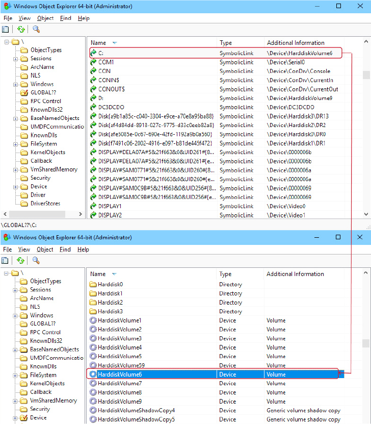
Figure 11-23 Drive-letter name resolution.

After locking the caller’s security context and obtaining security information from the caller’s token, IopParseDevice creates an I/O request packet (IRP) of type IRP_MJ_CREATE, creates a file object that stores the name of the file being opened, follows the VPB of the volume device object to find the volume’s mounted file system device object, and uses IoCallDriver to pass the IRP to the file system driver that owns the file system device object.

When an FSD receives an IRP_MJ_CREATE IRP, it looks up the specified file, performs security validation, and if the file exists and the user has permission to access the file in the way requested, returns a success status code. The object manager creates a handle for the file object in the process’s handle table, and the handle propagates back through the calling chain, finally reaching the application as a return parameter from CreateFile. If the file system fails the create operation, the I/O manager deletes the file object it created for the file.

We’ve skipped over the details of how the FSD locates the file being opened on the volume, but a ReadFile function call operation shares many of the FSD’s interactions with the cache manager and storage driver. Both ReadFile and CreateFile are system calls that map to I/O manager functions, but the NtReadFile system service doesn’t need to perform a name lookup; it calls on the object manager to translate the handle passed from ReadFile into a file object pointer. If the handle indicates that the caller obtained permission to read the file when the file was opened, NtReadFile proceeds to create an IRP of type IRP_MJ_READ and sends it to the FSD for the volume on which the file resides. NtReadFile obtains the FSD’s device object, which is stored in the file object, and calls IoCallDriver, and the I/O manager locates the FSD from the device object and gives the IRP to the FSD.

If the file being read can be cached (that is, the FILE_FLAG_NO_BUFFERING flag wasn’t passed to CreateFile when the file was opened), the FSD checks to see whether caching has already been initiated for the file object. The PrivateCacheMap field in a file object points to a private cache map data structure (which we described in the previous section) if caching is initiated for a file object. If the FSD hasn’t initialized caching for the file object (which it does the first time a file object is read from or written to), the PrivateCacheMap field will be null. The FSD calls the cache manager’s CcInitializeCacheMap function to initialize caching, which involves the cache manager creating a private cache map and, if another file object referring to the same file hasn’t initiated caching, a shared cache map and a section object.

After it has verified that caching is enabled for the file, the FSD copies the requested file data from the cache manager’s virtual memory to the buffer that the thread passed to the ReadFile function. The file system performs the copy within a try/except block so that it catches any faults that are the result of an invalid application buffer. The function the file system uses to perform the copy is the cache manager’s CcCopyRead function. CcCopyRead takes as parameters a file object, file offset, and length.

When the cache manager executes CcCopyRead, it retrieves a pointer to a shared cache map, which is stored in the file object. Recall that a shared cache map stores pointers to virtual address control blocks (VACBs), with one VACB entry for each 256 KB block of the file. If the VACB pointer for a portion of a file being read is null, CcCopyRead allocates a VACB, reserving a 256 KB view in the cache manager’s virtual address space, and maps (using MmMapViewInSystemCache) the specified portion of the file into the view. Then CcCopyRead simply copies the file data from the mapped view to the buffer it was passed (the buffer originally passed to ReadFile). If the file data isn’t in physical memory, the copy operation generates page faults, which are serviced by MmAccessFault.

When a page fault occurs, MmAccessFault examines the virtual address that caused the fault and locates the virtual address descriptor (VAD) in the VAD tree of the process that caused the fault. (See Chapter 5 of Part 1 for more information on VAD trees.) In this scenario, the VAD describes the cache manager’s mapped view of the file being read, so MmAccessFault calls MiDispatchFault to handle a page fault on a valid virtual memory address. MiDispatchFault locates the control area (which the VAD points to) and through the control area finds a file object representing the open file. (If the file has been opened more than once, there might be a list of file objects linked through pointers in their private cache maps.)

With the file object in hand, MiDispatchFault calls the I/O manager function IoPageRead to build an IRP (of type IRP_MJ_READ) and sends the IRP to the FSD that owns the device object the file object points to. Thus, the file system is reentered to read the data that it requested via CcCopyRead, but this time the IRP is marked as noncached and paging I/O. These flags signal the FSD that it should retrieve file data directly from disk, and it does so by determining which clusters on disk contain the requested data (the exact mechanism is file-system dependent) and sending IRPs to the volume manager that owns the volume device object on which the file resides. The volume parameter block (VPB) field in the FSD’s device object points to the volume device object.

The memory manager waits for the FSD to complete the IRP read and then returns control to the cache manager, which continues the copy operation that was interrupted by a page fault. When CcCopyRead completes, the FSD returns control to the thread that called NtReadFile, having copied the requested file data, with the aid of the cache manager and the memory manager, to the thread’s buffer.

The path for WriteFile is similar except that the NtWriteFile system service generates an IRP of type IRP_MJ_WRITE, and the FSD calls CcCopyWrite instead of CcCopyRead. CcCopyWrite, like CcCopyRead, ensures that the portions of the file being written are mapped into the cache and then copies to the cache the buffer passed to WriteFile.

If a file’s data is already cached (in the system’s working set), there are several variants on the scenario we’ve just described. If a file’s data is already stored in the cache, CcCopyRead doesn’t incur page faults. Also, under certain conditions, NtReadFile and NtWriteFile call an FSD’s fast I/O entry point instead of immediately building and sending an IRP to the FSD. Some of these conditions follow: the portion of the file being read must reside in the first 4 GB of the file, the file can have no locks, and the portion of the file being read or written must fall within the file’s currently allocated size.

The fast I/O read and write entry points for most FSDs call the cache manager’s CcFastCopyRead and CcFastCopyWrite functions. These variants on the standard copy routines ensure that the file’s data is mapped in the file system cache before performing a copy operation. If this condition isn’t met, CcFastCopyRead and CcFastCopyWrite indicate that fast I/O isn’t possible. When fast I/O isn’t possible, NtReadFile and NtWriteFile fall back on creating an IRP. (See the earlier section “Fast I/O” for a more complete description of fast I/O.)

Memory manager’s modified and mapped page writer

The memory manager’s modified and mapped page writer threads wake up periodically (and when available memory runs low) to flush modified pages to their backing store on disk. The threads call IoAsynchronousPageWrite to create IRPs of type IRP_MJ_WRITE and write pages to either a paging file or a file that was modified after being mapped. Like the IRPs that MiDispatchFault creates, these IRPs are flagged as noncached and paging I/O. Thus, an FSD bypasses the file system cache and issues IRPs directly to a storage driver to write the memory to disk.

Cache manager’s lazy writer

The cache manager’s lazy writer thread also plays a role in writing modified pages because it periodically flushes views of file sections mapped in the cache that it knows are dirty. The flush operation, which the cache manager performs by calling MmFlushSection, triggers the memory manager to write any modified pages in the portion of the section being flushed to disk. Like the modified and mapped page writers, MmFlushSection uses IoSynchronousPageWrite to send the data to the FSD.

Cache manager’s read-ahead thread

A cache uses two artifacts of how programs reference code and data: temporal locality and spatial locality. The underlying concept behind temporal locality is that if a memory location is referenced, it is likely to be referenced again soon. The idea behind spatial locality is that if a memory location is referenced, other nearby locations are also likely to be referenced soon. Thus, a cache typically is very good at speeding up access to memory locations that have been accessed in the near past, but it’s terrible at speeding up access to areas of memory that have not yet been accessed (it has zero lookahead capability). In an attempt to populate the cache with data that will likely be used soon, the cache manager implements two mechanisms: a read-ahead thread and Superfetch.

As we described in the previous section, the cache manager includes a thread that is responsible for attempting to read data from files before an application, a driver, or a system thread explicitly requests it. The read-ahead thread uses the history of read operations that were performed on a file, which are stored in a file object’s private cache map, to determine how much data to read. When the thread performs a read-ahead, it simply maps the portion of the file it wants to read into the cache (allocating VACBs as necessary) and touches the mapped data. The page faults caused by the memory accesses invoke the page fault handler, which reads the pages into the system’s working set.

A limitation of the read-ahead thread is that it works only on open files. Superfetch was added to Windows to proactively add files to the cache before they’re even opened. Specifically, the memory manager sends page-usage information to the Superfetch service (%SystemRoot%\System32\Sysmain.dll), and a file system minifilter provides file name resolution data. The Superfetch service attempts to find file-usage patterns—for example, payroll is run every Friday at 12:00, or Outlook is run every morning at 8:00. When these patterns are derived, the information is stored in a database and timers are requested. Just prior to the time the file would most likely be used, a timer fires and tells the memory manager to read the file into low-priority memory (using low-priority disk I/O). If the file is then opened, the data is already in memory, and there’s no need to wait for the data to be read from disk. If the file isn’t opened, the low-priority memory will be reclaimed by the system. The internals and full description of the Superfetch service were previously described in Chapter 5, Part 1.

Memory manager’s page fault handler

We described how the page fault handler is used in the context of explicit file I/O and cache manager read-ahead, but it’s also invoked whenever any application accesses virtual memory that is a view of a mapped file and encounters pages that represent portions of a file that aren’t yet in memory. The memory manager’s MmAccessFault handler follows the same steps it does when the cache manager generates a page fault from CcCopyRead or CcCopyWrite, sending IRPs via IoPageRead to the file system on which the file is stored.

File system filter drivers and minifilters

A filter driver that layers over a file system driver is called a file system filter driver. Two types of file system filter drivers are supported by the Windows I/O model:

• ■    Legacy file system filter drivers usually create one or multiple device objects and attach them on the file system device through the IoAttachDeviceToDeviceStack API. Legacy filter drivers intercept all the requests coming from the cache manager or I/O manager and must implement both standard IRP dispatch functions and the Fast I/O path. Due to the complexity involved in the development of this kind of driver (synchronization issues, undocumented interfaces, dependency on the original file system, and so on), Microsoft has developed a unified filter model that makes use of special drivers, called minifilters, and deprecated legacy file system drivers. (The IoAttachDeviceToDeviceStack API fails when it’s called for DAX volumes).

• ■    Minifilters drivers are clients of the Filesystem Filter Manager (Fltmgr.sys). The Filesystem Filter Manager is a legacy file system filter driver that provides a rich and documented interface for the creation of file system filters, hiding the complexity behind all the interactions between the file system drivers and the cache manager. Minifilters register with the filter manager through the FltRegisterFilter API. The caller usually specifies an instance setup routine and different operation callbacks. The instance setup is called by the filter manager for every valid volume device that a file system manages. The minifilter has the chance to decide whether to attach to the volume. Minifilters can specify a Pre and Post operation callback for every major IRP function code, as well as certain “pseudo-operations” that describe internal memory manager or cache manager semantics that are relevant to file system access patterns. The Pre callback is executed before the I/O is processed by the file system driver, whereas the Post callback is executed after the I/O operation has been completed. The Filter Manager also provides its own communication facility that can be employed between minifilter drivers and their associated user-mode application.

The ability to see all file system requests and optionally modify or complete them enables a range of applications, including remote file replication services, file encryption, efficient backup, and licensing. Every anti-malware product typically includes at least a minifilter driver that intercepts applications opening or modifying files. For example, before propagating the IRP to the file system driver to which the command is directed, a malware scanner examines the file being opened to ensure that it’s clean. If the file is clean, the malware scanner passes the IRP on, but if the file is infected, the malware scanner quarantines or cleans the file. If the file can’t be cleaned, the driver fails the IRP (typically with an access-denied error) so that the malware cannot become active.

Deeply describing the entire minifilter and legacy filter driver architecture is outside the scope of this chapter. You can find more information on the legacy filter driver architecture in Chapter 6, “I/O System,” of Part 1. More details on minifilters are available in MSDN (https://docs.microsoft.com/en-us/windows-hardware/drivers/ifs/file-system-minifilter-drivers).

Data-scan sections

Starting with Windows 8.1, the Filter Manager collaborates with file system drivers to provide data-scan section objects that can be used by anti-malware products. Data-scan section objects are similar to standard section objects (for more information about section objects, see Chapter 5 of Part 1) except for the following:

• ■    Data-scan section objects can be created from minifilter callback functions, namely from callbacks that manage the IRP_MJ_CREATE function code. These callbacks are called by the filter manager when an application is opening or creating a file. An anti-malware scanner can create a data-scan section and then start scanning before completing the callback.

• ■    FltCreateSectionForDataScan, the API used for creating data-scan sections, accepts a FILE_OBJECT pointer. This means that callers don’t need to provide a file handle. The file handle typically doesn’t yet exist, and would thus need to be (re)created by using FltCreateFile API, which would then have created other file creation IRPs, recursively interacting with lower level file system filters once again. With the new API, the process is much faster because these extra recursive calls won’t be generated.

A data-scan section can be mapped like a normal section using the traditional API. This allows anti-malware applications to implement their scan engine either as a user-mode application or in a kernel-mode driver. When the data-scan section is mapped, IRP_MJ_READ events are still generated in the minifilter driver, but this is not a problem because the minifilter doesn’t have to include a read callback at all.

Filtering named pipes and mailslots

When a process belonging to a user application needs to communicate with another entity (a process, kernel driver, or remote application), it can leverage facilities provided by the operating system. The most traditionally used are named pipes and mailslots, because they are portable among other operating systems as well. A named pipe is a named, one-way communication channel between a pipe server and one or more pipe clients. All instances of a named pipe share the same pipe name, but each instance has its own buffers and handles, and provides a separate channel for client/server communication. Named pipes are implemented through a file system driver, the NPFS driver (Npfs.sys).

A mailslot is a multi-way communication channel between a mailslot server and one or more clients. A mailslot server is a process that creates a mailslot through the CreateMailslot Win32 API, and can only read small messages (424 bytes maximum when sent between remote computers) generated by one or more clients. Clients are processes that write messages to the mailslot. Clients connect to the mailslot through the standard CreateFile API and send messages through the WriteFile function. Mailslots are generally used for broadcasting messages within a domain. If several server processes in a domain each create a mailslot using the same name, every message that is addressed to that mailslot and sent to the domain is received by the participating processes. Mailslots are implemented through the Mailslot file system driver, Msfs.sys.

Both the mailslot and NPFS driver implement simple file systems. They manage namespaces composed of files and directories, which support security, can be opened, closed, read, written, and so on. Describing the implementation of the two drivers is outside the scope of this chapter.

Starting with Windows 8, mailslots and named pipes are supported by the Filter Manager. Minifilters are able to attach to the mailslot and named pipe volumes (\Device\NamedPipe and \Device\Mailslot, which are not real volumes), through the FLTFL_REGISTRATION_SUPPORT_NPFS_MSFS flag specified at registration time. A minifilter can then intercept and modify all the named pipe and mailslot I/O that happens between local and remote process and between a user application and its kernel driver. Furthermore, minifilters can open or create a named pipe or mailslot without generating recursive events through the FltCreateNamedPipeFile or FltCreateMailslotFile APIs.

Note

One of the motivations that explains why the named pipe and mailslot file system drivers are simpler compared to NTFS and ReFs is that they do not interact heavily with the cache manager. The named pipe driver implements the Fast I/O path but with no cached read or write-behind support. The mailslot driver does not interact with the cache manager at all.

Controlling reparse point behavior

The NTFS file system supports the concept of reparse points, blocks of 16 KB of application and system-defined reparse data that can be associated to single files. (Reparse points are discussed more in multiple sections later in this chapter.) Some types of reparse points, like volume mount points or symbolic links, contain a link between the original file (or an empty directory), used as a placeholder, and another file, which can even be located in another volume. When the NTFS file system driver encounters a reparse point on its path, it returns an error code to the upper driver in the device stack. The latter (which could be another filter driver) analyzes the reparse point content and, in the case of a symbolic link, re-emits another I/O to the correct volume device.

This process is complex and cumbersome for any filter driver. Minifilters drivers can intercept the STATUS_REPARSE error code and reopen the reparse point through the new FltCreateFileEx2 API, which accepts a list of Extra Create Parameters (also known as ECPs), used to fine-tune the behavior of the opening/creation process of a target file in the minifilter context. In general, the Filter Manager supports different ECPs, and each of them is uniquely identified by a GUID. The Filter Manager provides multiple documented APIs that deal with ECPs and ECP lists. Usually, minifilters allocate an ECP with the FltAllocateExtraCreateParameter function, populate it, and insert it into a list (through FltInsertExtraCreateParameter) before calling the Filter Manager’s I/O APIs.

The FLT_CREATEFILE_TARGET extra creation parameter allows the Filter Manager to manage cross-volume file creation automatically (the caller needs to specify a flag). Minifilters don’t need to perform any other complex operation.

With the goal of supporting container isolation, it’s also possible to set a reparse point on nonempty directories and, in order to support container isolation, create new files that have directory reparse points. The default behavior that the file system has while encountering a nonempty directory reparse point depends on whether the reparse point is applied in the last component of the file full path. If this is the case, the file system returns the STATUS_REPARSE error code, just like for an empty directory; otherwise, it continues to walk the path.

The Filter Manager is able to correctly deal with this new kind of reparse point through another ECP (named TYPE_OPEN_REPARSE). The ECP includes a list of descriptors (OPEN_REPARSE_LIST_ ENTRY data structure), each of which describes the type of reparse point (through its Reparse Tag), and the behavior that the system should apply when it encounters a reparse point of that type while parsing a path. Minifilters, after they have correctly initialized the descriptor list, can apply the new behavior in different ways:

• ■    Issue a new open (or create) operation on a file that resides in a path that includes a reparse point in any of its components, using the FltCreateFileEx2 function. This procedure is similar to the one used by the FLT_CREATEFILE_TARGET ECP.

• ■    Apply the new reparse point behavior globally to any file that the Pre-Create callback intercepts. The FltAddOpenReparseEntry and FltRemoveOpenReparseEntry APIs can be used to set the reparse point behavior to a target file before the file is actually created (the pre-creation callback intercepts the file creation request before the file is created). The Windows Container Isolation minifilter driver (Wcifs.sys) uses this strategy.

Process Monitor

Process Monitor (Procmon), a system activity-monitoring utility from Sysinternals that has been used throughout this book, is an example of a passive minifilter driver, which is one that does not modify the flow of IRPs between applications and file system drivers.

Process Monitor works by extracting a file system minifilter device driver from its executable image (stored as a resource inside Procmon.exe) the first time you run it after a boot, installing the driver in memory, and then deleting the driver image from disk (unless configured for persistent boot-time monitoring). Through the Process Monitor GUI, you can direct the driver to monitor file system activity on local volumes that have assigned drive letters, network shares, named pipes, and mail slots. When the driver receives a command to start monitoring a volume, it registers filtering callbacks with the Filter Manager, which is attached to the device object that represents a mounted file system on the volume. After an attach operation, the I/O manager redirects an IRP targeted at the underlying device object to the driver owning the attached device, in this case the Filter Manager, which sends the event to registered minifilter drivers, in this case Process Monitor.

When the Process Monitor driver intercepts an IRP, it records information about the IRP’s command, including target file name and other parameters specific to the command (such as read and write lengths and offsets) to a nonpaged kernel buffer. Every 500 milliseconds, the Process Monitor GUI program sends an IRP to Process Monitor’s interface device object, which requests a copy of the buffer containing the latest activity, and then displays the activity in its output window. Process Monitor shows all file activity as it occurs, which makes it an ideal tool for troubleshooting file system–related system and application failures. To run Process Monitor the first time on a system, an account must have the Load Driver and Debug privileges. After loading, the driver remains resident, so subsequent executions require only the Debug privilege.

When you run Process Monitor, it starts in basic mode, which shows the file system activity most often useful for troubleshooting. When in basic mode, Process Monitor omits certain file system operations from being displayed, including

• ■    I/O to NTFS metadata files

• ■    I/O to the paging file

• ■    I/O generated by the System process

• ■    I/O generated by the Process Monitor process

While in basic mode, Process Monitor also reports file I/O operations with friendly names rather than with the IRP types used to represent them. For example, both IRP_MJ_WRITE and FASTIO_WRITE operations display as WriteFile, and IRP_MJ_CREATE operations show as Open if they represent an open operation and as Create for the creation of new files.

EXPERIMENT: Viewing Process Monitor’s minifilter driver

To see which file system minifilter drivers are loaded, start an Administrative command prompt, and run the Filter Manager control program (%SystemRoot%\System32\Fltmc.exe). Start Process Monitor (ProcMon.exe) and run Fltmc again. You see that the Process Monitor’s filter driver (PROCMON20) is loaded and has a nonzero value in the Instances column. Now, exit Process Monitor and run Fltmc again. This time, you see that the Process Monitor’s filter driver is still loaded, but now its instance count is zero.

The NT File System (NTFS)

In the following section, we analyze the internal architecture of the NTFS file system, starting by looking at the requirements that drove its design. We examine the on-disk data structures, and then we move on to the advanced features provided by the NTFS file system, like the Recovery support, tiered volumes, and the Encrypting File System (EFS).

High-end file system requirements

From the start, NTFS was designed to include features required of an enterprise-class file system. To minimize data loss in the face of an unexpected system outage or crash, a file system must ensure that the integrity of its metadata is guaranteed at all times; and to protect sensitive data from unauthorized access, a file system must have an integrated security model. Finally, a file system must allow for software-based data redundancy as a low-cost alternative to hardware-redundant solutions for protecting user data. In this section, you find out how NTFS implements each of these capabilities.

Recoverability

To address the requirement for reliable data storage and data access, NTFS provides file system recovery based on the concept of an atomic transaction. Atomic transactions are a technique for handling modifications to a database so that system failures don’t affect the correctness or integrity of the database. The basic tenet of atomic transactions is that some database operations, called transactions, are all-or-nothing propositions. (A transaction is defined as an I/O operation that alters file system data or changes the volume’s directory structure.) The separate disk updates that make up the transaction must be executed atomically—that is, once the transaction begins to execute, all its disk updates must be completed. If a system failure interrupts the transaction, the part that has been completed must be undone, or rolled back. The rollback operation returns the database to a previously known and consistent state, as if the transaction had never occurred.

NTFS uses atomic transactions to implement its file system recovery feature. If a program initiates an I/O operation that alters the structure of an NTFS volume—that is, changes the directory structure, extends a file, allocates space for a new file, and so on—NTFS treats that operation as an atomic transaction. It guarantees that the transaction is either completed or, if the system fails while executing the transaction, rolled back. The details of how NTFS does this are explained in the section “NTFS recovery support” later in the chapter. In addition, NTFS uses redundant storage for vital file system information so that if a sector on the disk goes bad, NTFS can still access the volume’s critical file system data.

Security

Security in NTFS is derived directly from the Windows object model. Files and directories are protected from being accessed by unauthorized users. (For more information on Windows security, see Chapter 7, “Security,” in Part 1.) An open file is implemented as a file object with a security descriptor stored on disk in the hidden $Secure metafile, in a stream named $SDS (Security Descriptor Stream). Before a process can open a handle to any object, including a file object, the Windows security system verifies that the process has appropriate authorization to do so. The security descriptor, combined with the requirement that a user log on to the system and provide an identifying password, ensures that no process can access a file unless it is given specific permission to do so by a system administrator or by the file’s owner. (For more information about security descriptors, see the section “Security descriptors and access control” in Chapter 7 in Part 1).

Data redundancy and fault tolerance

In addition to recoverability of file system data, some customers require that their data not be endangered by a power outage or catastrophic disk failure. The NTFS recovery capabilities ensure that the file system on a volume remains accessible, but they make no guarantees for complete recovery of user files. Protection for applications that can’t risk losing file data is provided through data redundancy.

Data redundancy for user files is implemented via the Windows layered driver, which provides fault-tolerant disk support. NTFS communicates with a volume manager, which in turn communicates with a disk driver to write data to a disk. A volume manager can mirror, or duplicate, data from one disk onto another disk so that a redundant copy can always be retrieved. This support is commonly called RAID level 1. Volume managers also allow data to be written in stripes across three or more disks, using the equivalent of one disk to maintain parity information. If the data on one disk is lost or becomes inaccessible, the driver can reconstruct the disk’s contents by means of exclusive-OR operations. This support is called RAID level 5.

In Windows 7, data redundancy for NTFS implemented via the Windows layered driver was provided by Dynamic Disks. Dynamic Disks had multiple limitations, which have been overcome in Windows 8.1 by introducing a new technology that virtualizes the storage hardware, called Storage Spaces. Storage Spaces is able to create virtual disks that already provide data redundancy and fault tolerance. The volume manager doesn’t differentiate between a virtual disk and a real disk (so user mode components can’t see any difference between the two). The NTFS file system driver cooperates with Storage Spaces for supporting tiered disks and RAID virtual configurations. Storage Spaces and Spaces Direct will be covered later in this chapter.

Advanced features of NTFS

In addition to NTFS being recoverable, secure, reliable, and efficient for mission-critical systems, it includes the following advanced features that allow it to support a broad range of applications. Some of these features are exposed as APIs for applications to leverage, and others are internal features:

• ■    Multiple data streams

• ■    Unicode-based names

• ■    General indexing facility

• ■    Dynamic bad-cluster remapping

• ■    Hard links

• ■    Symbolic (soft) links and junctions

• ■    Compression and sparse files

• ■    Change logging

• ■    Per-user volume quotas

• ■    Link tracking

• ■    Encryption

• ■    POSIX support

• ■    Defragmentation

• ■    Read-only support and dynamic partitioning

• ■    Tiered volume support

The following sections provide an overview of these features.

Multiple data streams

In NTFS, each unit of information associated with a file—including its name, its owner, its time stamps, its contents, and so on—is implemented as a file attribute (NTFS object attribute). Each attribute consists of a single stream—that is, a simple sequence of bytes. This generic implementation makes it easy to add more attributes (and therefore more streams) to a file. Because a file’s data is “just another attribute” of the file and because new attributes can be added, NTFS files (and file directories) can contain multiple data streams.

An NTFS file has one default data stream, which has no name. An application can create additional, named data streams and access them by referring to their names. To avoid altering the Windows I/O APIs, which take a string as a file name argument, the name of the data stream is specified by appending a colon (:) to the file name. Because the colon is a reserved character, it can serve as a separator between the file name and the data stream name, as illustrated in this example:

myfile.dat:stream2

Each stream has a separate allocation size (which defines how much disk space has been reserved for it), actual size (which is how many bytes the caller has used), and valid data length (which is how much of the stream has been initialized). In addition, each stream is given a separate file lock that is used to lock byte ranges and to allow concurrent access.

One component in Windows that uses multiple data streams is the Attachment Execution Service, which is invoked whenever the standard Windows API for saving internet-based attachments is used by applications such as Edge or Outlook. Depending on which zone the file was downloaded from (such as the My Computer zone, the Intranet zone, or the Untrusted zone), Windows Explorer might warn the user that the file came from a possibly untrusted location or even completely block access to the file. For example, Figure 11-24 shows the dialog box that’s displayed when executing Process Explorer after it was downloaded from the Sysinternals site. This type of data stream is called the $Zone.Identifier and is colloquially referred to as the “Mark of the Web.”

Figure 11-24 Security warning for files downloaded from the internet.

Note

If you clear the check box for Always Ask Before Opening This File, the zone identifier data stream will be removed from the file.

Other applications can use the multiple data stream feature as well. A backup utility, for example, might use an extra data stream to store backup-specific time stamps on files. Or an archival utility might implement hierarchical storage in which files that are older than a certain date or that haven’t been accessed for a specified period of time are moved to offline storage. The utility could copy the file to offline storage, set the file’s default data stream to 0, and add a data stream that specifies where the file is stored.

EXPERIMENT: Looking at streams

Most Windows applications aren’t designed to work with alternate named streams, but both the echo and more commands are. Thus, a simple way to view streams in action is to create a named stream using echo and then display it using more. The following command sequence creates a file named test with a stream named stream:

Click here to view code image

c:\Test>echo Hello from a named stream! > test:stream
    c:\Test>more < test:stream
    Hello from a named stream!
    
    c:\Test>

If you perform a directory listing, Test’s file size doesn’t reflect the data stored in the alternate stream because NTFS returns the size of only the unnamed data stream for file query operations, including directory listings.

Click here to view code image

c:\Test>dir test
     Volume in drive C is OS.
     Volume Serial Number is F080-620F
    
     Directory of c:\Test
    
    12/07/2018  05:33 PM                 0 test
                   1 File(s)              0 bytes
                   0 Dir(s)  18,083,577,856 bytes free
    c:\Test>

You can determine what files and directories on your system have alternate data streams with the Streams utility from Sysinternals (see the following output) or by using the /r switch in the dir command.

Click here to view code image

c:\Test>streams test
    
    streams v1.60 - Reveal NTFS alternate streams.
    Copyright (C) 2005-2016 Mark Russinovich
    Sysinternals - www.sysinternals.com
    
    c:\Test\test:
              :stream:$DATA 29

Unicode-based names

Like Windows as a whole, NTFS supports 16-bit Unicode 1.0/UTF-16 characters to store names of files, directories, and volumes. Unicode allows each character in each of the world’s major languages to be uniquely represented (Unicode can even represent emoji, or small drawings), which aids in moving data easily from one country to another. Unicode is an improvement over the traditional representation of international characters—using a double-byte coding scheme that stores some characters in 8 bits and others in 16 bits, a technique that requires loading various code pages to establish the available characters. Because Unicode has a unique representation for each character, it doesn’t depend on which code page is loaded. Each directory and file name in a path can be as many as 255 characters long and can contain Unicode characters, embedded spaces, and multiple periods.

General indexing facility

The NTFS architecture is structured to allow indexing of any file attribute on a disk volume using a B-tree structure. (Creating indexes on arbitrary attributes is not exported to users.) This structure enables the file system to efficiently locate files that match certain criteria—for example, all the files in a particular directory. In contrast, the FAT file system indexes file names but doesn’t sort them, making lookups in large directories slow.

Several NTFS features take advantage of general indexing, including consolidated security descriptors, in which the security descriptors of a volume’s files and directories are stored in a single internal stream, have duplicates removed, and are indexed using an internal security identifier that NTFS defines. The use of indexing by these features is described in the section “NTFS on-disk structure” later in this chapter.

Dynamic bad-cluster remapping

Ordinarily, if a program tries to read data from a bad disk sector, the read operation fails and the data in the allocated cluster becomes inaccessible. If the disk is formatted as a fault-tolerant NTFS volume, however, the Windows volume manager—or Storage Spaces, depending on the component that provides data redundancy—dynamically retrieves a good copy of the data that was stored on the bad sector and then sends NTFS a warning that the sector is bad. NTFS will then allocate a new cluster, replacing the cluster in which the bad sector resides, and copies the data to the new cluster. It adds the bad cluster to the list of bad clusters on that volume (stored in the hidden metadata file $BadClus) and no longer uses it. This data recovery and dynamic bad-cluster remapping is an especially useful feature for file servers and fault-tolerant systems or for any application that can’t afford to lose data. If the volume manager or Storage Spaces is not used when a sector goes bad (such as early in the boot sequence), NTFS still replaces the cluster and doesn’t reuse it, but it can’t recover the data that was on the bad sector.

Hard links

A hard link allows multiple paths to refer to the same file. (Hard links are not supported on directories.) If you create a hard link named C:\Documents\Spec.doc that refers to the existing file C:\Users \Administrator\Documents\Spec.doc, the two paths link to the same on-disk file, and you can make changes to the file using either path. Processes can create hard links with the Windows CreateHardLink function.

NTFS implements hard links by keeping a reference count on the actual data, where each time a hard link is created for the file, an additional file name reference is made to the data. This means that if you have multiple hard links for a file, you can delete the original file name that referenced the data (C:\Users\Administrator\Documents\Spec.doc in our example), and the other hard links (C:\Documents\Spec.doc) will remain and point to the data. However, because hard links are on-disk local references to data (represented by a file record number), they can exist only within the same volume and can’t span volumes or computers.

EXPERIMENT: Creating a hard link

There are two ways you can create a hard link: the fsutil hardlink create command or the mklink utility with the /H option. In this experiment we’ll use mklink because we’ll use this utility later to create a symbolic link as well. First, create a file called test.txt and add some text to it, as shown here.

Click here to view code image

C:\>echo Hello from a Hard Link > test.txt

Now create a hard link called hard.txt as shown here:

Click here to view code image

C:\>mklink hard.txt test.txt /H
    Hardlink created for hard.txt <<===>> test.txt

If you list the directory’s contents, you’ll notice that the two files will be identical in every way, with the same creation date, permissions, and file size; only the file names differ.

Click here to view code image

c:\>dir *.txt
     Volume in drive C is OS
     Volume Serial Number is F080-620F
    
     Directory of c:\
    
    12/07/2018  05:46 PM                26 hard.txt
    12/07/2018  05:46 PM                26 test.txt
                   2 File(s)             52 bytes
                   0 Dir(s)  15,150,333,952 bytes free

Symbolic (soft) links and junctions

In addition to hard links, NTFS supports another type of file-name aliasing called symbolic links or soft links. Unlike hard links, symbolic links are strings that are interpreted dynamically and can be relative or absolute paths that refer to locations on any storage device, including ones on a different local volume or even a share on a different system. This means that symbolic links don’t actually increase the reference count of the original file, so deleting the original file will result in the loss of the data, and a symbolic link that points to a nonexisting file will be left behind. Finally, unlike hard links, symbolic links can point to directories, not just files, which gives them an added advantage.

For example, if the path C:\Drivers is a directory symbolic link that redirects to %SystemRoot%\System32\Drivers, an application reading C:\Drivers\Ntfs.sys actually reads %SystemRoot%\System\Drivers\Ntfs.sys. Directory symbolic links are a useful way to lift directories that are deep in a directory tree to a more convenient depth without disturbing the original tree’s structure or contents. The example just cited lifts the Drivers directory to the volume’s root directory, reducing the directory depth of Ntfs.sys from three levels to one when Ntfs.sys is accessed through the directory symbolic link. File symbolic links work much the same way—you can think of them as shortcuts, except they’re actually implemented on the file system instead of being .lnk files managed by Windows Explorer. Just like hard links, symbolic links can be created with the mklink utility (without the /H option) or through the CreateSymbolicLink API.

Because certain legacy applications might not behave securely in the presence of symbolic links, especially across different machines, the creation of symbolic links requires the SeCreateSymbolicLink privilege, which is typically granted only to administrators. Starting with Windows 10, and only if Developer Mode is enabled, callers of CreateSymbolicLink API can additionally specify the SYMBOLIC_LINK_FLAG_ ALLOW_UNPRIVILEGED_CREATE flag to overcome this limitation (this allows a standard user is still able to create symbolic links from the command prompt window). The file system also has a behavior option called SymLinkEvaluation that can be configured with the following command:

Click here to view code image

fsutil behavior set SymLinkEvaluation

By default, the Windows default symbolic link evaluation policy allows only local-to-local and local-to-remote symbolic links but not the opposite, as shown here:

Click here to view code image

D:\>fsutil behavior query SymLinkEvaluation
    Local to local symbolic links are enabled
    Local to remote symbolic links are enabled.
    Remote to local symbolic links are disabled.
    Remote to Remote symbolic links are disabled.

Symbolic links are implemented using an NTFS mechanism called reparse points. (Reparse points are discussed further in the section “Reparse points” later in this chapter.) A reparse point is a file or directory that has a block of data called reparse data associated with it. Reparse data is user-defined data about the file or directory, such as its state or location that can be read from the reparse point by the application that created the data, a file system filter driver, or the I/O manager. When NTFS encounters a reparse point during a file or directory lookup, it returns the STATUS_REPARSE status code, which signals file system filter drivers that are attached to the volume and the I/O manager to examine the reparse data. Each reparse point type has a unique reparse tag. The reparse tag allows the component responsible for interpreting the reparse point’s reparse data to recognize the reparse point without having to check the reparse data. A reparse tag owner, either a file system filter driver or the I/O manager, can choose one of the following options when it recognizes reparse data:

• ■    The reparse tag owner can manipulate the path name specified in the file I/O operation that crosses the reparse point and let the I/O operation reissue with the altered path name. Junctions (described shortly) take this approach to redirect a directory lookup, for example.

• ■    The reparse tag owner can remove the reparse point from the file, alter the file in some way, and then reissue the file I/O operation.

There are no Windows functions for creating reparse points. Instead, processes must use the FSCTL_SET_REPARSE_POINT file system control code with the Windows DeviceIoControl function. A process can query a reparse point’s contents with the FSCTL_GET_REPARSE_POINT file system control code. The FILE_ATTRIBUTE_REPARSE_POINT flag is set in a reparse point’s file attributes, so applications can check for reparse points by using the Windows GetFileAttributes function.

Another type of reparse point that NTFS supports is the junction (also known as Volume Mount point). Junctions are a legacy NTFS concept and work almost identically to directory symbolic links, except they can only be local to a volume. There is no advantage to using a junction instead of a directory symbolic link, except that junctions are compatible with older versions of Windows, while directory symbolic links are not.

As seen in the previous section, modern versions of Windows now allow the creation of reparse points that can point to non-empty directories. The system behavior (which can be controlled from minifilters drivers) depends on the position of the reparse point in the target file’s full path. The filter manager, NTFS, and ReFS file system drivers use the exposed FsRtlIsNonEmptyDirectoryReparsePointAllowed API to detect if a reparse point type is allowed on non-empty directories.

EXPERIMENT: Creating a symbolic link

This experiment shows you the main difference between a symbolic link and a hard link, even when dealing with files on the same volume. Create a symbolic link called soft.txt as shown here, pointing to the test.txt file created in the previous experiment:

Click here to view code image

C:\>mklink soft.txt test.txt
    symbolic link created for soft.txt <<===>> test.txt

If you list the directory’s contents, you’ll notice that the symbolic link doesn’t have a file size and is identified by the <SYMLINK> type. Furthermore, you’ll note that the creation time is that of the symbolic link, not of the target file. The symbolic link can also have security permissions that are different from the permissions on the target file.

Click here to view code image

C:\>dir *.txt
     Volume in drive C is OS
     Volume Serial Number is 38D4-EA71
    
     Directory of C:\
    
    05/12/2012  11:55 PM                 8 hard.txt
    05/13/2012  12:28 AM    <SYMLINK>      soft.txt [test.txt]
    05/12/2012  11:55 PM                 8 test.txt
                   3 File(s)             16 bytes
                   0 Dir(s)  10,636,480,512 bytes free

Finally, if you delete the original test.txt file, you can verify that both the hard link and symbolic link still exist but that the symbolic link does not point to a valid file anymore, while the hard link references the file data.

Compression and sparse files

NTFS supports compression of file data. Because NTFS performs compression and decompression procedures transparently, applications don’t have to be modified to take advantage of this feature. Directories can also be compressed, which means that any files subsequently created in the directory are compressed.

Applications compress and decompress files by passing DeviceIoControl the FSCTL_SET_COMPRESSION file system control code. They query the compression state of a file or directory with the FSCTL_GET_COMPRESSION file system control code. A file or directory that is compressed has the FILE_ATTRIBUTE_COMPRESSED flag set in its attributes, so applications can also determine a file or directory’s compression state with GetFileAttributes.

A second type of compression is known as sparse files. If a file is marked as sparse, NTFS doesn’t allocate space on a volume for portions of the file that an application designates as empty. NTFS returns 0-filled buffers when an application reads from empty areas of a sparse file. This type of compression can be useful for client/server applications that implement circular-buffer logging, in which the server records information to a file, and clients asynchronously read the information. Because the information that the server writes isn’t needed after a client has read it, there’s no need to store the information in the file. By making such a file sparse, the client can specify the portions of the file it reads as empty, freeing up space on the volume. The server can continue to append new information to the file without fear that the file will grow to consume all available space on the volume.

As with compressed files, NTFS manages sparse files transparently. Applications specify a file’s sparseness state by passing the FSCTL_SET_SPARSE file system control code to DeviceIoControl. To set a range of a file to empty, applications use the FSCTL_SET_ZERO_DATA code, and they can ask NTFS for a description of what parts of a file are sparse by using the control code FSCTL_QUERY_ALLOCATED _RANGES. One application of sparse files is the NTFS change journal, described next.

Change logging

Many types of applications need to monitor volumes for file and directory changes. For example, an automatic backup program might perform an initial full backup and then incremental backups based on file changes. An obvious way for an application to monitor a volume for changes is for it to scan the volume, recording the state of files and directories, and on a subsequent scan detect differences. This process can adversely affect system performance, however, especially on computers with thousands or tens of thousands of files.

An alternate approach is for an application to register a directory notification by using the FindFirstChangeNotification or ReadDirectoryChangesW Windows function. As an input parameter, the application specifies the name of a directory it wants to monitor, and the function returns whenever the contents of the directory change. Although this approach is more efficient than volume scanning, it requires the application to be running at all times. Using these functions can also require an application to scan directories because FindFirstChangeNotification doesn’t indicate what changed—just that something in the directory has changed. An application can pass a buffer to ReadDirectoryChangesW that the FSD fills in with change records. If the buffer overflows, however, the application must be prepared to fall back on scanning the directory.

NTFS provides a third approach that overcomes the drawbacks of the first two: an application can configure the NTFS change journal facility by using the DeviceIoControl function’s FSCTL_CREATE_USN_ JOURNAL file system control code (USN is update sequence number) to have NTFS record information about file and directory changes to an internal file called the change journal. A change journal is usually large enough to virtually guarantee that applications get a chance to process changes without missing any. Applications use the FSCTL_QUERY_USN_JOURNAL file system control code to read records from a change journal, and they can specify that the DeviceIoControl function not complete until new records are available.

Per-user volume quotas

Systems administrators often need to track or limit user disk space usage on shared storage volumes, so NTFS includes quota-management support. NTFS quota-management support allows for per-user specification of quota enforcement, which is useful for usage tracking and tracking when a user reaches warning and limit thresholds. NTFS can be configured to log an event indicating the occurrence to the System event log if a user surpasses his warning limit. Similarly, if a user attempts to use more volume storage then her quota limit permits, NTFS can log an event to the System event log and fail the application file I/O that would have caused the quota violation with a “disk full” error code.

NTFS tracks a user’s volume usage by relying on the fact that it tags files and directories with the security ID (SID) of the user who created them. (See Chapter 7, “Security,” in Part 1 for a definition of SIDs.) The logical sizes of files and directories a user owns count against the user’s administrator-defined quota limit. Thus, a user can’t circumvent his or her quota limit by creating an empty sparse file that is larger than the quota would allow and then fill the file with nonzero data. Similarly, whereas a 50 KB file might compress to 10 KB, the full 50 KB is used for quota accounting.

By default, volumes don’t have quota tracking enabled. You need to use the Quota tab of a volume’s Properties dialog box, shown in Figure 11-25, to enable quotas, to specify default warning and limit thresholds, and to configure the NTFS behavior that occurs when a user hits the warning or limit threshold. The Quota Entries tool, which you can launch from this dialog box, enables an administrator to specify different limits and behavior for each user. Applications that want to interact with NTFS quota management use COM quota interfaces, including IDiskQuotaControl, IDiskQuotaUser, and IDiskQuotaEvents.

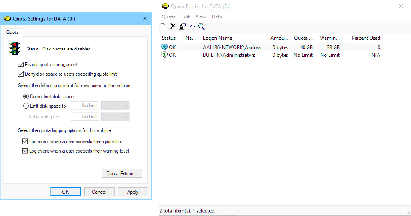
Figure 11-25 The Quota Settings dialog accessible from the volume’s Properties window.

Link tracking

Shell shortcuts allow users to place files in their shell namespaces (on their desktops, for example) that link to files located in the file system namespace. The Windows Start menu uses shell shortcuts extensively. Similarly, object linking and embedding (OLE) links allow documents from one application to be transparently embedded in the documents of other applications. The products of the Microsoft Office suite, including PowerPoint, Excel, and Word, use OLE linking.

Although shell and OLE links provide an easy way to connect files with one another and with the shell namespace, they can be difficult to manage if a user moves the source of a shell or OLE link (a link source is the file or directory to which a link points). NTFS in Windows includes support for a service application called distributed link-tracking, which maintains the integrity of shell and OLE links when link targets move. Using the NTFS link-tracking support, if a link target located on an NTFS volume moves to any other NTFS volume within the originating volume’s domain, the link-tracking service can transparently follow the movement and update the link to reflect the change.

NTFS link-tracking support is based on an optional file attribute known as an object ID. An application can assign an object ID to a file by using the FSCTL_CREATE_OR_GET_OBJECT_ID (which assigns an ID if one isn’t already assigned) and FSCTL_SET_OBJECT_ID file system control codes. Object IDs are queried with the FSCTL_CREATE_OR_GET_OBJECT_ID and FSCTL_GET_OBJECT_ID file system control codes. The FSCTL_DELETE_OBJECT_ID file system control code lets applications delete object IDs from files.

Encryption

Corporate users often store sensitive information on their computers. Although data stored on company servers is usually safely protected with proper network security settings and physical access control, data stored on laptops can be exposed when a laptop is lost or stolen. NTFS file permissions don’t offer protection because NTFS volumes can be fully accessed without regard to security by using NTFS file-reading software that doesn’t require Windows to be running. Furthermore, NTFS file permissions are rendered useless when an alternate Windows installation is used to access files from an administrator account. Recall from Chapter 6 in Part 1 that the administrator account has the take-ownership and backup privileges, both of which allow it to access any secured object by overriding the object’s security settings.

NTFS includes a facility called Encrypting File System (EFS), which users can use to encrypt sensitive data. The operation of EFS, as that of file compression, is completely transparent to applications, which means that file data is automatically decrypted when an application running in the account of a user authorized to view the data reads it and is automatically encrypted when an authorized application changes the data.

Note

NTFS doesn’t permit the encryption of files located in the system volume’s root directory or in the \Windows directory because many files in these locations are required during the boot process, and EFS isn’t active during the boot process. BitLocker is a technology much better suited for environments in which this is a requirement because it supports full-volume encryption. As we will describe in the next paragraphs, Bitlocker collaborates with NTFS for supporting file-encryption.

EFS relies on cryptographic services supplied by Windows in user mode, so it consists of both a kernel-mode component that tightly integrates with NTFS as well as user-mode DLLs that communicate with the Local Security Authority Subsystem (LSASS) and cryptographic DLLs.

Files that are encrypted can be accessed only by using the private key of an account’s EFS private/public key pair, and private keys are locked using an account’s password. Thus, EFS-encrypted files on lost or stolen laptops can’t be accessed using any means (other than a brute-force cryptographic attack) without the password of an account that is authorized to view the data.

Applications can use the EncryptFile and DecryptFile Windows API functions to encrypt and decrypt files, and FileEncryptionStatus to retrieve a file or directory’s EFS-related attributes, such as whether the file or directory is encrypted. A file or directory that is encrypted has the FILE_ATTRIBUTE_ENCRYPTED flag set in its attributes, so applications can also determine a file or directory’s encryption state with GetFileAttributes.

POSIX-style delete semantics

The POSIX Subsystem has been deprecated and is no longer available in the Windows operating system. The Windows Subsystem for Linux (WSL) has replaced the original POSIX Subsystem. The NTFS file system driver has been updated to unify the differences between I/O operations supported in Windows and those supported in Linux. One of these differences is provided by the Linux unlink (or rm) command, which deletes a file or a folder. In Windows, an application can’t delete a file that is in use by another application (which has an open handle to it); conversely, Linux usually supports this: other processes continue to work well with the original deleted file. To support WSL, the NTFS file system driver in Windows 10 supports a new operation: POSIX Delete.

The Win32 DeleteFile API implements standard file deletion. The target file is opened (a new handle is created), and then a disposition label is attached to the file through the NtSetInformationFile native API. The label just communicates to the NTFS file system driver that the file is going to be deleted. The file system driver checks whether the number of references to the FCB (File Control Block) is equal to 1, meaning that there is no other outstanding open handle to the file. If so, the file system driver marks the file as “deleted on close” and then returns. Only when the handle to the file is closed does the IRP_MJ_CLEANUP dispatch routine physically remove the file from the underlying medium.

A similar architecture is not compatible with the Linux unlink command. The WSL subsystem, when it needs to erase a file, employs POSIX-style deletion; it calls the NtSetInformationFile native API with the new FileDispositionInformationEx information class, specifying a flag (FILE_DISPOSITION_POSIX_SEMANTICS). The NTFS file system driver marks the file as POSIX deleted by inserting a flag in its Context Control Block (CCB, a data structure that represents the context of an open instance of an on-disk object). It then re-opens the file with a special internal routine and attaches the new handle (which we will call the PosixDeleted handle) to the SCB (stream control block). When the original handle is closed, the NTFS file system driver detects the presence of the PosixDeleted handle and queues a work item for closing it. When the work item completes, the Cleanup routine detects that the handle is marked as POSIX delete and physically moves the file in the “\$Extend\$Deleted” hidden directory. Other applications can still operate on the original file, which is no longer in the original namespace and will be deleted only when the last file handle is closed (the first delete request has marked the FCB as delete-on-close).

If for any unusual reason the system is not able to delete the target file (due to a dangling reference in a defective kernel driver or due to a sudden power interruption), the next time that the NTFS file system has the chance to mount the volume, it checks the \$Extend\$Deleted directory and deletes every file included in it by using standard file deletion routines.

Note

Starting with the May 2019 Update (19H1), Windows 10 now uses POSIX delete as the default file deletion method. This means that the DeleteFile API uses the new behavior.

EXPERIMENT: Witnessing POSIX delete

In this experiment, you’re going to witness a POSIX delete through the FsTool application, which is available in this book’s downloadable resources. Make sure you’re using a copy of Windows Server 2019 (RS5). Indeed, newer client releases of Windows implement POSIX deletions by default. Start by opening a command prompt window. Use the /touch FsTool command-line argument to generate a txt file that’s exclusively used by the application:

Click here to view code image

D:\>FsTool.exe /touch d:\Test.txt
    NTFS / ReFS Tool v0.1
    Copyright (C) 2018 Andrea Allievi (AaLl86)
    
    Touching "d:\Test.txt" file... Success.
       The File handle is valid... Press Enter to write to the file.

When requested, instead of pressing the Enter key, open another command prompt window and try to open and delete the file:

Click here to view code image

D:\>type Test.txt
    The process cannot access the file because it is being used by another process.
    
    D:\>del Test.txt
    
    D:\>dir Test.txt
     Volume in drive D is DATA
     Volume Serial Number is 62C1-9EB3
    
     Directory of D:\
    
    12/13/2018  12:34 AM                49 Test.txt
                   1 File(s)             49 bytes
                   0 Dir(s)  1,486,254,481,408 bytes free

As expected, you can’t open the file while FsTool has exclusive access to it. When you try to delete the file, the system marks it for deletion, but it’s not able to remove it from the file system namespace. If you try to delete the file again with File Explorer, you can witness the same behavior. When you press Enter in the first command prompt window and you exit the FsTool application, the file is actually deleted by the NTFS file system driver.

The next step is to use a POSIX deletion for getting rid of the file. You can do this by specifying the /pdel command-line argument to the FsTool application. In the first command prompt window, restart FsTool with the /touch command-line argument (the original file has been already marked for deletion, and you can’t delete it again). Before pressing Enter, switch to the second window and execute the following command:

Click here to view code image

D:\>FsTool /pdel Test.txt
    NTFS / ReFS Tool v0.1
    Copyright (C) 2018 Andrea Allievi (AaLl86)
    
    Deleting "Test.txt" file (Posix semantics)... Success.
    Press any key to exit...
    
    D:\>dir Test.txt
     Volume in drive D is DATA
     Volume Serial Number is 62C1-9EB3
    
     Directory of D:\
    
    File Not Found

In this case the Test.txt file has been completely removed from the file system’s namespace but is still valid. If you press Enter in the first command prompt window, FsTool is still able to write data to the file. This is because the file has been internally moved into the \$Extend\$Deleted hidden system directory.

Defragmentation

Even though NTFS makes efforts to keep files contiguous when allocating blocks to extend a file, a volume’s files can still become fragmented over time, especially if the file is extended multiple times or when there is limited free space. A file is fragmented if its data occupies discontiguous clusters. For example, Figure 11-26 shows a fragmented file consisting of five fragments. However, like most file systems (including versions of FAT on Windows), NTFS makes no special efforts to keep files contiguous (this is handled by the built-in defragmenter), other than to reserve a region of disk space known as the master file table (MFT) zone for the MFT. (NTFS lets other files allocate from the MFT zone when volume free space runs low.) Keeping an area free for the MFT can help it stay contiguous, but it, too, can become fragmented. (See the section “Master file table” later in this chapter for more information on MFTs.)

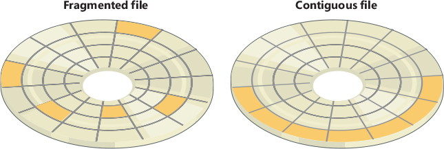
Figure 11-26 Fragmented and contiguous files.

To facilitate the development of third-party disk defragmentation tools, Windows includes a defragmentation API that such tools can use to move file data so that files occupy contiguous clusters. The API consists of file system controls that let applications obtain a map of a volume’s free and in-use clusters (FSCTL_GET_VOLUME_BITMAP), obtain a map of a file’s cluster usage (FSCTL_GET_RETRIEVAL_POINTERS), and move a file (FSCTL_MOVE_FILE).

Windows includes a built-in defragmentation tool that is accessible by using the Optimize Drives utility (%SystemRoot%\System32\Dfrgui.exe), shown in Figure 11-27, as well as a command-line interface, %SystemRoot%\System32\Defrag.exe, that you can run interactively or schedule, but that does not produce detailed reports or offer control—such as excluding files or directories—over the defragmentation process.

Figure 11-27 The Optimize Drives tool.

The only limitation imposed by the defragmentation implementation in NTFS is that paging files and NTFS log files can’t be defragmented. The Optimize Drives tool is the evolution of the Disk Defragmenter, which was available in Windows 7. The tool has been updated to support tiered volumes, SMR disks, and SSD disks. The optimization engine is implemented in the Optimize Drive service (Defragsvc.dll), which exposes the IDefragEngine COM interface used by both the graphical tool and the command-line interface.

For SSD disks, the tool also implements the retrim operation. To understand the retrim operation, a quick introduction of the architecture of a solid-state drive is needed. SSD disks store data in flash memory cells that are grouped into pages of 4 to 16 KB, grouped together into blocks of typically 128 to 512 pages. Flash memory cells can only be directly written to when they’re empty. If they contain data, the contents must be erased before a write operation. An SSD write operation can be done on a single page but, due to hardware limitations, erase commands always affect entire blocks; consequently, writing data to empty pages on an SSD is very fast but slows down considerably once previously written pages need to be overwritten. (In this case, first the content of the entire block is stored in cache, and then the entire block is erased from the SSD. The overwritten page is written to the cached block, and finally the entire updated block is written to the flash medium.) To overcome this problem, the NTFS File System Driver tries to send a TRIM command to the SSD controller every time it deletes the disk’s clusters (which could partially or entirely belong to a file). In response to the TRIM command, the SSD, if possible, starts to asynchronously erase entire blocks. Noteworthy is that the SSD controller can’t do anything in case the deleted area corresponds only to some pages of the block.

The retrim operation analyzes the SSD disk and starts to send a TRIM command to every cluster in the free space (in chunks of 1-MB size). There are different motivations behind this:

• ■    TRIM commands are not always emitted. (The file system is not very strict on trims.)

• ■    The NTFS File System emits TRIM commands on pages, but not on SSD blocks. The Disk Optimizer, with the retrim operation, searches fragmented blocks. For those blocks, it first moves valid data back to some temporary blocks, defragmenting the original ones and inserting even pages that belongs to other fragmented blocks; finally, it emits TRIM commands on the original cleaned blocks.

Note

The way in which the Disk Optimizer emits TRIM commands on free space is somewhat tricky: Disk Optimizer allocates an empty sparse file and searches for a chunk (the size of which varies from 128 KB to 1 GB) of free space. It then calls the file system through the FSCTL_MOVE_FILE control code and moves data from the sparse file (which has a size of 1 GB but does not actually contain any valid data) into the empty space. The underlying file system actually erases the content of the one or more SSD blocks (sparse files with no valid data yield back chunks of zeroed data when read). This is the implementation of the TRIM command that the SSD firmware does.

For Tiered and SMR disks, the Optimize Drives tool supports two supplementary operations: Slabify (also known as Slab Consolidation) and Tier Optimization. Big files stored on tiered volumes can be composed of different Extents residing in different tiers. The Slab consolidation operation not only defragments the extent table (a phase called Consolidation) of a file, but it also moves the file content in congruent slabs (a slab is a unit of allocation of a thinly provisioned disk; see the “Storage Spaces” section later in this chapter for more information). The final goal of Slab Consolidation is to allow files to use a smaller number of slabs. Tier Optimization moves frequently accessed files (including files that have been explicitly pinned) from the capacity tier to the performance tier and, vice versa, moves less frequently accessed files from the performance tier to the capacity tier. To do so, the optimization engine consults the tiering engine, which provides file extents that should be moved to the capacity tier and those that should be moved to the performance tier, based on the Heat map for every file accessed by the user.

Note

Tiered disks and the tiering engine are covered in detail in the following sections of the current chapter.

EXPERIMENT: Retrim an SSD volume

You can execute a Retrim on a fast SSD or NVMe volume by using the defrag.exe /L command, as in the following example:

Click here to view code image

D:\>defrag /L c:
    Microsoft Drive Optimizer
    Copyright (c) Microsoft Corp.
    
    Invoking retrim on (C:)...
    
    The operation completed successfully.
    
    Post Defragmentation Report:
    
            Volume Information:
                   Volume size                  = 475.87 GB
                    Free space                  = 343.80 GB
    
            Retrim:
                    Total space trimmed         = 341.05 GB

In the example, the volume size was 475.87 GB, with 343.80 GB of free space. Only 341 GB have been erased and trimmed. Obviously, if you execute the command on volumes backed by a classical HDD, you will get back an error. (The operation requested is not supported by the hardware backing the volume.)

Dynamic partitioning

The NTFS driver allows users to dynamically resize any partition, including the system partition, either shrinking or expanding it (if enough space is available). Expanding a partition is easy if enough space exists on the disk and the expansion is performed through the FSCTL_EXPAND_VOLUME file system control code. Shrinking a partition is a more complicated process because it requires moving any file system data that is currently in the area to be thrown away to the region that will still remain after the shrinking process (a mechanism similar to defragmentation). Shrinking is implemented by two components: the shrinking engine and the file system driver.

The shrinking engine is implemented in user mode. It communicates with NTFS to determine the maximum number of reclaimable bytes—that is, how much data can be moved from the region that will be resized into the region that will remain. The shrinking engine uses the standard defragmentation mechanism shown earlier, which doesn’t support relocating page file fragments that are in use or any other files that have been marked as unmovable with the FSCTL_MARK_HANDLE file system control code (like the hibernation file). The master file table backup ($MftMirr), the NTFS metadata transaction log ($LogFile), and the volume label file ($Volume) cannot be moved, which limits the minimum size of the shrunk volume and causes wasted space.

The file system driver shrinking code is responsible for ensuring that the volume remains in a consistent state throughout the shrinking process. To do so, it exposes an interface that uses three requests that describe the current operation, which are sent through the FSCTL_SHRINK_VOLUME control code:

• ■    The ShrinkPrepare request, which must be issued before any other operation. This request takes the desired size of the new volume in sectors and is used so that the file system can block further allocations outside the new volume boundary. The ShrinkPrepare request doesn’t verify whether the volume can actually be shrunk by the specified amount, but it does ensure that the amount is numerically valid and that there aren’t any other shrinking operations ongoing. Note that after a prepare operation, the file handle to the volume becomes associated with the shrink request. If the file handle is closed, the operation is assumed to be aborted.

• ■    The ShrinkCommit request, which the shrinking engine issues after a ShrinkPrepare request. In this state, the file system attempts the removal of the requested number of clusters in the most recent prepare request. (If multiple prepare requests have been sent with different sizes, the last one is the determining one.) The ShrinkCommit request assumes that the shrinking engine has completed and will fail if any allocated blocks remain in the area to be shrunk.

• ■    The ShrinkAbort request, which can be issued by the shrinking engine or caused by events such as the closure of the file handle to the volume. This request undoes the ShrinkCommit operation by returning the partition to its original size and allows new allocations outside the shrunk region to occur again. However, defragmentation changes made by the shrinking engine remain.

If a system is rebooted during a shrinking operation, NTFS restores the file system to a consistent state via its metadata recovery mechanism, explained later in the chapter. Because the actual shrink operation isn’t executed until all other operations have been completed, the volume retains its original size and only defragmentation operations that had already been flushed out to disk persist.

Finally, shrinking a volume has several effects on the volume shadow copy mechanism. Recall that the copy-on-write mechanism allows VSS to simply retain parts of the file that were actually modified while still linking to the original file data. For deleted files, this file data will not be associated with visible files but appears as free space instead—free space that will likely be located in the area that is about to be shrunk. The shrinking engine therefore communicates with VSS to engage it in the shrinking process. In summary, the VSS mechanism’s job is to copy deleted file data into its differencing area and to increase the differencing area as required to accommodate additional data. This detail is important because it poses another constraint on the size to which even volumes with ample free space can shrink.

NTFS support for tiered volumes

Tiered volumes are composed of different types of storage devices and underlying media. Tiered volumes are usually created on the top of a single physical or virtual disk. Storage Spaces provides virtual disks that are composed of multiple physical disks, which can be of different types (and have different performance): fast NVMe disks, SSD, and Rotating Hard-Disk. A virtual disk of this type is called a tiered disk. (Storage Spaces uses the name Storage Tiers.) On the other hand, tiered volumes could be created on the top of physical SMR disks, which have a conventional “random-access” fast zone and a “strictly sequential” capacity area. All tiered volumes have the common characteristic that they are composed by a “performance” tier, which supports fast random I/O, and a “capacity” tier, which may or may not support random I/O, is slower, and has a large capacity.

Note

SMR disks, tiered volumes, and Storage Spaces will be discussed in more detail later in this chapter.

The NTFS File System driver supports tiered volumes in multiple ways:

• ■    The volume is split in two zones, which correspond to the tiered disk areas (capacity and performance).

• ■    The new $DSC attribute (of type $LOGGED_UTILITY_STREAM) specifies which tier the file should be stored in. NTFS exposes a new “pinning” interface, which allows a file to be locked in a particular tier (from here derives the term “pinning”) and prevents the file from being moved by the tiering engine.

• ■    The Storage Tiers Management service has a central role in supporting tiered volumes. The NTFS file system driver records ETW “heat” events every time a file stream is read or written. The tiering engine consumes these events, accumulates them (in 1-MB chunks), and periodically records them in a JET database (once every hour). Every four hours, the tiering engine processes the Heat database and through a complex “heat aging” algorithm decides which file is considered recent (hot) and which is considered old (cold). The tiering engine moves the files between the performance and the capacity tiers based on the calculated Heat data.

Furthermore, the NTFS allocator has been modified to allocate file clusters based on the tier area that has been specified in the $DSC attribute. The NTFS Allocator uses a specific algorithm to decide from which tier to allocate the volume’s clusters. The algorithm operates by performing checks in the following order:

1. If the file is the Volume USN Journal, always allocate from the Capacity tier.

2. MFT entries (File Records) and system metadata files are always allocated from the Performance tier.

3. If the file has been previously explicitly “pinned” (meaning that the file has the $DSC attribute), allocate from the specified storage tier.

4. If the system runs a client edition of Windows, always prefer the Performance tier; otherwise, allocate from the Capacity tier.

5. If there is no space in the Performance tier, allocate from the Capacity tier.

An application can specify the desired storage tier for a file by using the NtSetInformationFile API with the FileDesiredStorageClassInformation information class. This operation is called file pinning, and, if executed on a handle of a new created file, the central allocator will allocate the new file content in the specified tier. Otherwise, if the file already exists and is located on the wrong tier, the tiering engine will move the file to the desired tier the next time it runs. (This operation is called Tier optimization and can be initiated by the Tiering Engine scheduled task or the SchedulerDefrag task.)

Note

It’s important to note here that the support for tiered volumes in NTFS, described here, is completely different from the support provided by the ReFS file system driver.

EXPERIMENT: Witnessing file pinning in tiered volumes

As we have described in the previous section, the NTFS allocator uses a specific algorithm to decide which tier to allocate from. In this experiment, you copy a big file into a tiered volume and understand what the implications of the File Pinning operation are. After the copy finishes, open an administrative PowerShell window by right-clicking on the Start menu icon and selecting Windows PowerShell (Admin) and use the Get-FileStorageTier command to get the tier information for the file:

Click here to view code image

PS E:\> Get-FileStorageTier -FilePath 'E:\Big_Image.iso' | FL FileSize,
    DesiredStorageTierClass, FileSizeOnPerformanceTierClass, FileSizeOnCapacityTierClass,
    PlacementStatus, State
    
    FileSize                       : 4556566528
    DesiredStorageTierClass        : Unknown
    FileSizeOnPerformanceTierClass : 0
    FileSizeOnCapacityTierClass    : 4556566528
    PlacementStatus                : Unknown
    State                          : Unknown

The example shows that the Big_Image.iso file has been allocated from the Capacity Tier. (The example has been executed on a Windows Server system.) To confirm this, just copy the file from the tiered disk to a fast SSD volume. You should see a slow transfer speed (usually between 160 and 250 MB/s depending on the rotating disk speed):

You can now execute the “pin” request through the Set-FileStorageTier command, like in the following example:

Click here to view code image

PS E:\> Get-StorageTier -MediaType SSD | FL FriendlyName, Size, FootprintOnPool, UniqueId
    
    FriendlyName    : SSD
    Size            : 128849018880
    FootprintOnPool : 128849018880
    UniqueId        : {448abab8-f00b-42d6-b345-c8da68869020}
    
    PS E:\> Set-FileStorageTier -FilePath 'E:\Big_Image.iso' -DesiredStorageTierFriendlyName
    'SSD'
    PS E:\> Get-FileStorageTier -FilePath 'E:\Big_Image.iso' | FL FileSize,
    DesiredStorageTierClass, FileSizeOnPerformanceTierClass, FileSizeOnCapacityTierClass,
    PlacementStatus, State
    
    FileSize                       : 4556566528
    DesiredStorageTierClass        : Performance
    FileSizeOnPerformanceTierClass : 0
    FileSizeOnCapacityTierClass    : 4556566528
    PlacementStatus                : Not on tier
    State                          : Pending

The example above shows that the file has been correctly pinned on the Performance tier, but its content is still stored in the Capacity tier. When the Tiering Engine scheduled task runs, it moves the file extents from the Capacity to the Performance tier. You can force a Tier Optimization by running the Drive optimizer through the defrag.exe /g built-in tool:

Click here to view code image

PS E:> defrag /g /h e:
    Microsoft Drive Optimizer
    Copyright (c) Microsoft Corp.
    
    Invoking tier optimization on Test (E:)...
    
    
    Pre-Optimization Report:
    
            Volume Information:
                    Volume size                 = 2.22 TB
                    Free space                  = 1.64 TB
                    Total fragmented space      = 36%
                    Largest free space size     = 1.56 TB
    
            Note: File fragments larger than 64MB are not included in the fragmentation statistics.
    
    The operation completed successfully.
    
    Post Defragmentation Report:
    
            Volume Information:
                    Volume size                 = 2.22 TB
                    Free space                  = 1.64 TB
    
            Storage Tier Optimization Report:
    
                    % I/Os Serviced from Perf Tier  Perf Tier Size Required
                    100%                            28.51 GB *
                    95%                             22.86 GB
    ...
                    20%                             2.44 GB
                    15%                             1.58 GB
                    10%                             873.80 MB
                    5%                              361.28 MB
    
            * Current size of the Performance tier: 474.98 GB
              Percent of total I/Os serviced from the Performance tier: 99%
    
            Size of files pinned to the Performance tier: 4.21 GB
            Percent of total I/Os: 1%
    
            Size of files pinned to the Capacity tier: 0 bytes
            Percent of total I/Os: 0%

The Drive Optimizer has confirmed the “pinning” of the file. You can check again the “pinning” status by executing the Get-FileStorageTier command and by copying the file again to an SSD volume. This time the transfer rate should be much higher, because the file content is entirely located in the Performance tier.

Click here to view code image

PS E:\> Get-FileStorageTier -FilePath 'E:\Big_Image.iso' | FL FileSize, DesiredStorageTierClass,
    FileSizeOnPerformanceTierClass, FileSizeOnCapacityTierClass, PlacementStatus, State
    
    FileSize                       : 4556566528
    DesiredStorageTierClass        : Performance
    FileSizeOnPerformanceTierClass : 0
    FileSizeOnCapacityTierClass    : 4556566528
    PlacementStatus                : Completely on tier
    State                          : OK

You could repeat the experiment in a client edition of Windows 10, by pinning the file in the Capacity tier (client editions of Windows 10 allocate file’s clusters from the Performance tier by default). The same “pinning” functionality has been implemented into the FsTool application available in this book’s downloadable resources, which can be used to copy a file directly into a preferred tier.

NTFS file system driver

As described in Chapter 6 in Part I, in the framework of the Windows I/O system, NTFS and other file systems are loadable device drivers that run in kernel mode. They are invoked indirectly by applications that use Windows or other I/O APIs. As Figure 11-28 shows, the Windows environment subsystems call Windows system services, which in turn locate the appropriate loaded drivers and call them. (For a description of system service dispatching, see the section “System service dispatching” in Chapter 8.)

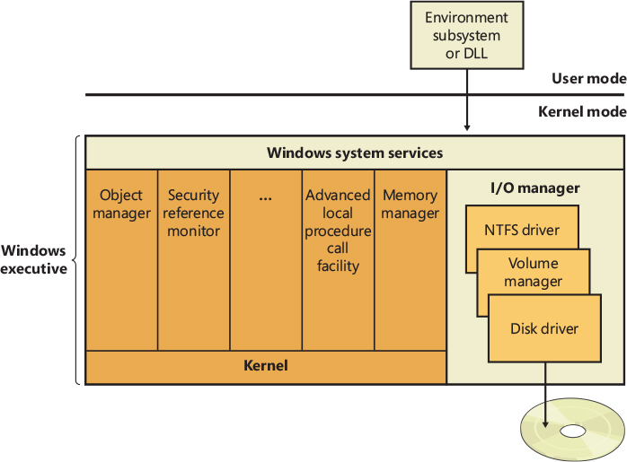
Figure 11-28 Components of the Windows I/O system.

The layered drivers pass I/O requests to one another by calling the Windows executive’s I/O manager. Relying on the I/O manager as an intermediary allows each driver to maintain independence so that it can be loaded or unloaded without affecting other drivers. In addition, the NTFS driver interacts with the three other Windows executive components, shown in the left side of Figure 11-29, which are closely related to file systems.

The log file service (LFS) is the part of NTFS that provides services for maintaining a log of disk writes. The log file that LFS writes is used to recover an NTFS-formatted volume in the case of a system failure. (See the section “Log file service” later in this chapter.)

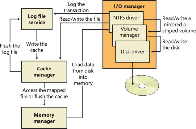
Figure 11-29 NTFS and related components.

As we have already described, the cache manager is the component of the Windows executive that provides systemwide caching services for NTFS and other file system drivers, including network file system drivers (servers and redirectors). All file systems implemented for Windows access cached files by mapping them into system address space and then accessing the virtual memory. The cache manager provides a specialized file system interface to the Windows memory manager for this purpose. When a program tries to access a part of a file that isn’t loaded into the cache (a cache miss), the memory manager calls NTFS to access the disk driver and obtain the file contents from disk. The cache manager optimizes disk I/O by using its lazy writer threads to call the memory manager to flush cache contents to disk as a background activity (asynchronous disk writing).

NTFS, like other file systems, participates in the Windows object model by implementing files as objects. This implementation allows files to be shared and protected by the object manager, the component of Windows that manages all executive-level objects. (The object manager is described in the section “Object manager” in Chapter 8.)

An application creates and accesses files just as it does other Windows objects: by means of object handles. By the time an I/O request reaches NTFS, the Windows object manager and security system have already verified that the calling process has the authority to access the file object in the way it is attempting to. The security system has compared the caller’s access token to the entries in the access control list for the file object. (See Chapter 7 in Part 1 for more information about access control lists.) The I/O manager has also transformed the file handle into a pointer to a file object. NTFS uses the information in the file object to access the file on disk.

Figure 11-30 shows the data structures that link a file handle to the file system’s on-disk structure.

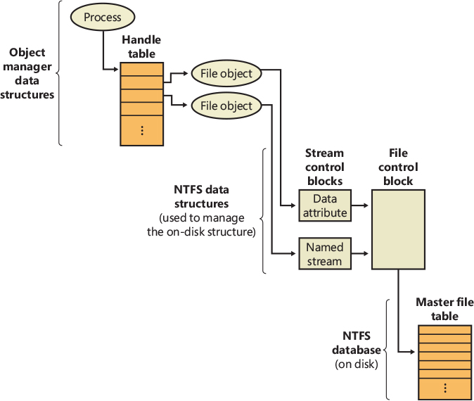
Figure 11-30 NTFS data structures.

NTFS follows several pointers to get from the file object to the location of the file on disk. As Figure 11-30 shows, a file object, which represents a single call to the open-file system service, points to a stream control block (SCB) for the file attribute that the caller is trying to read or write. In Figure 11-30, a process has opened both the unnamed data attribute and a named stream (alternate data attribute) for the file. The SCBs represent individual file attributes and contain information about how to find specific attributes within a file. All the SCBs for a file point to a common data structure called a file control block (FCB). The FCB contains a pointer (actually, an index into the MFT, as explained in the section “File record numbers” later in this chapter) to the file’s record in the disk-based master file table (MFT), which is described in detail in the following section.

NTFS on-disk structure

This section describes the on-disk structure of an NTFS volume, including how disk space is divided and organized into clusters, how files are organized into directories, how the actual file data and attribute information is stored on disk, and finally, how NTFS data compression works.

Volumes

The structure of NTFS begins with a volume. A volume corresponds to a logical partition on a disk, and it’s created when you format a disk or part of a disk for NTFS. You can also create a RAID virtual disk that spans multiple physical disks by using Storage Spaces, which is accessible through the Manage Storage Spaces control panel snap-in, or by using Storage Spaces commands available from the Windows PowerShell (like the New-StoragePool command, used to create a new storage pool. A comprehensive list of PowerShell commands for Storage Spaces is available at the following link: https://docs.microsoft.com/en-us/powershell/module/storagespaces/)

A disk can have one volume or several. NTFS handles each volume independently of the others. Three sample disk configurations for a 2-TB hard disk are illustrated in Figure 11-31.

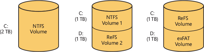
Figure 11-31 Sample disk configurations.

A volume consists of a series of files plus any additional unallocated space remaining on the disk partition. In all FAT file systems, a volume also contains areas specially formatted for use by the file system. An NTFS or ReFS volume, however, stores all file system data, such as bitmaps and directories, and even the system bootstrap, as ordinary files.

Note

The on-disk format of NTFS volumes on Windows 10 and Windows Server 2019 is version 3.1, the same as it has been since Windows XP and Windows Server 2003. The version number of a volume is stored in its $Volume metadata file.

Clusters

The cluster size on an NTFS volume, or the cluster factor, is established when a user formats the volume with either the format command or the Disk Management MMC snap-in. The default cluster factor varies with the size of the volume, but it is an integral number of physical sectors, always a power of 2 (1 sector, 2 sectors, 4 sectors, 8 sectors, and so on). The cluster factor is expressed as the number of bytes in the cluster, such as 512 bytes, 1 KB, 2 KB, and so on.

Internally, NTFS refers only to clusters. (However, NTFS forms low-level volume I/O operations such that clusters are sector-aligned and have a length that is a multiple of the sector size.) NTFS uses the cluster as its unit of allocation to maintain its independence from physical sector sizes. This independence allows NTFS to efficiently support very large disks by using a larger cluster factor or to support newer disks that have a sector size other than 512 bytes. On a larger volume, use of a larger cluster factor can reduce fragmentation and speed allocation, at the cost of wasted disk space. (If the cluster size is 64 KB, and a file is only 16 KB, then 48 KB are wasted.) Both the format command available from the command prompt and the Format menu option under the All Tasks option on the Action menu in the Disk Management MMC snap-in choose a default cluster factor based on the volume size, but you can override this size.

NTFS refers to physical locations on a disk by means of logical cluster numbers (LCNs). LCNs are simply the numbering of all clusters from the beginning of the volume to the end. To convert an LCN to a physical disk address, NTFS multiplies the LCN by the cluster factor to get the physical byte offset on the volume, as the disk driver interface requires. NTFS refers to the data within a file by means of virtual cluster numbers (VCNs). VCNs number the clusters belonging to a particular file from 0 through m. VCNs aren’t necessarily physically contiguous, however; they can be mapped to any number of LCNs on the volume.

Master file table

In NTFS, all data stored on a volume is contained in files, including the data structures used to locate and retrieve files, the bootstrap data, and the bitmap that records the allocation state of the entire volume (the NTFS metadata). Storing everything in files allows the file system to easily locate and maintain the data, and each separate file can be protected by a security descriptor. In addition, if a particular part of the disk goes bad, NTFS can relocate the metadata files to prevent the disk from becoming inaccessible.

The MFT is the heart of the NTFS volume structure. The MFT is implemented as an array of file records. The size of each file record can be 1 KB or 4 KB, as defined at volume-format time, and depends on the type of the underlying physical medium: new physical disks that have 4 KB native sectors size and tiered disks generally use 4 KB file records, while older disks that have 512 bytes sectors size use 1 KB file records. The size of each MFT entry does not depend on the clusters size and can be overridden at volume-format time through the Format /l command. (The structure of a file record is described in the “File records” section later in this chapter.) Logically, the MFT contains one record for each file on the volume, including a record for the MFT itself. In addition to the MFT, each NTFS volume includes a set of metadata files containing the information that is used to implement the file system structure. Each of these NTFS metadata files has a name that begins with a dollar sign ($) and is hidden. For example, the file name of the MFT is $MFT. The rest of the files on an NTFS volume are normal user files and directories, as shown in Figure 11-32.

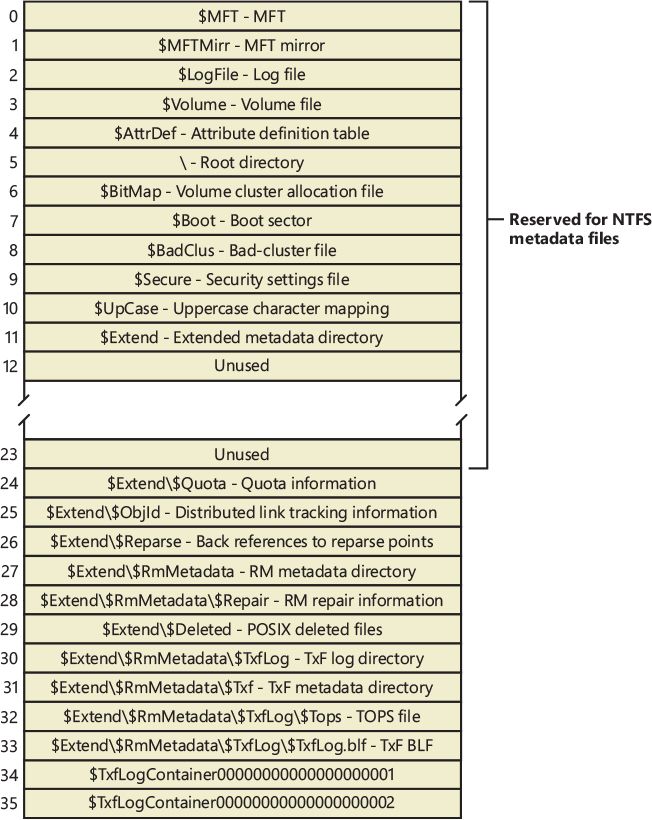
Figure 11-32 File records for NTFS metadata files in the MFT.

Usually, each MFT record corresponds to a different file. If a file has a large number of attributes or becomes highly fragmented, however, more than one record might be needed for a single file. In such cases, the first MFT record, which stores the locations of the others, is called the base file record.

When it first accesses a volume, NTFS must mount it—that is, read metadata from the disk and construct internal data structures so that it can process application file system accesses. To mount the volume, NTFS looks in the volume boot record (VBR) (located at LCN 0), which contains a data structure called the boot parameter block (BPB), to find the physical disk address of the MFT. The MFT’s file record is the first entry in the table; the second file record points to a file located in the middle of the disk called the MFT mirror (file name $MFTMirr) that contains a copy of the first four rows of the MFT. This partial copy of the MFT is used to locate metadata files if part of the MFT file can’t be read for some reason.

Once NTFS finds the file record for the MFT, it obtains the VCN-to-LCN mapping information in the file record’s data attribute and stores it into memory. Each run (runs are explained later in this chapter in the section “Resident and nonresident attributes”) has a VCN-to-LCN mapping and a run length because that’s all the information necessary to locate the LCN for any VCN. This mapping information tells NTFS where the runs containing the MFT are located on the disk. NTFS then processes the MFT records for several more metadata files and opens the files. Next, NTFS performs its file system recovery operation (described in the section “Recovery” later in this chapter), and finally, it opens its remaining metadata files. The volume is now ready for user access.

Note

For the sake of clarity, the text and diagrams in this chapter depict a run as including a VCN, an LCN, and a run length. NTFS actually compresses this information on disk into an LCN/next-VCN pair. Given a starting VCN, NTFS can determine the length of a run by subtracting the starting VCN from the next VCN.

As the system runs, NTFS writes to another important metadata file, the log file (file name $LogFile). NTFS uses the log file to record all operations that affect the NTFS volume structure, including file creation or any commands, such as copy, that alter the directory structure. The log file is used to recover an NTFS volume after a system failure and is also described in the “Recovery” section.

Another entry in the MFT is reserved for the root directory (also known as \; for example, C:\). Its file record contains an index of the files and directories stored in the root of the NTFS directory structure. When NTFS is first asked to open a file, it begins its search for the file in the root directory’s file record. After opening a file, NTFS stores the file’s MFT record number so that it can directly access the file’s MFT record when it reads and writes the file later.

NTFS records the allocation state of the volume in the bitmap file (file name $BitMap). The data attribute for the bitmap file contains a bitmap, each of whose bits represents a cluster on the volume, identifying whether the cluster is free or has been allocated to a file.

The security file (file name $Secure) stores the volume-wide security descriptor database. NTFS files and directories have individually settable security descriptors, but to conserve space, NTFS stores the settings in a common file, which allows files and directories that have the same security settings to reference the same security descriptor. In most environments, entire directory trees have the same security settings, so this optimization provides a significant saving of disk space.

Another system file, the boot file (file name $Boot), stores the Windows bootstrap code if the volume is a system volume. On nonsystem volumes, there is code that displays an error message on the screen if an attempt is made to boot from that volume. For the system to boot, the bootstrap code must be located at a specific disk address so that the Boot Manager can find it. During formatting, the format command defines this area as a file by creating a file record for it. All files are in the MFT, and all clusters are either free or allocated to a file—there are no hidden files or clusters in NTFS, although some files (metadata) are not visible to users. The boot file as well as NTFS metadata files can be individually protected by means of the security descriptors that are applied to all Windows objects. Using this “everything on the disk is a file” model also means that the bootstrap can be modified by normal file I/O, although the boot file is protected from editing.

NTFS also maintains a bad-cluster file (file name $BadClus) for recording any bad spots on the disk volume and a file known as the volume file (file name $Volume), which contains the volume name, the version of NTFS for which the volume is formatted, and a number of flag bits that indicate the state and health of the volume, such as a bit that indicates that the volume is corrupt and must be repaired by the Chkdsk utility. (The Chkdsk utility is covered in more detail later in the chapter.) The uppercase file (file name $UpCase) includes a translation table between lowercase and uppercase characters. NTFS maintains a file containing an attribute definition table (file name $AttrDef) that defines the attribute types supported on the volume and indicates whether they can be indexed, recovered during a system recovery operation, and so on.

Note

Figure 11-32 shows the Master File Table of a NTFS volume and indicates the specific entries in which the metadata files are located. It is worth mentioning that file records at position less than 16 are guaranteed to be fixed. Metadata files located at entries greater than 16 are subject to the order in which NTFS creates them. Indeed, the format tool doesn’t create any metadata file above position 16; this is the duty of the NTFS file system driver while mounting the volume for the first time (after the formatting has been completed). The order of the metadata files generated by the file system driver is not guaranteed.

NTFS stores several metadata files in the extensions (directory name $Extend) metadata directory, including the object identifier file (file name $ObjId), the quota file (file name $Quota), the change journal file (file name $UsnJrnl), the reparse point file (file name $Reparse), the Posix delete support directory ($Deleted), and the default resource manager directory (directory name $RmMetadata). These files store information related to extended features of NTFS. The object identifier file stores file object IDs, the quota file stores quota limit and behavior information on volumes that have quotas enabled, the change journal file records file and directory changes, and the reparse point file stores information about which files and directories on the volume include reparse point data.

The Posix Delete directory ($Deleted) contains files, which are invisible to the user, that have been deleted using the new Posix semantic. Files deleted using the Posix semantic will be moved in this directory when the application that has originally requested the file deletion closes the file handle. Other applications that may still have a valid reference to the file continue to run while the file’s name is deleted from the namespace. Detailed information about the Posix deletion has been provided in the previous section.

The default resource manager directory contains directories related to transactional NTFS (TxF) support, including the transaction log directory (directory name $TxfLog), the transaction isolation directory (directory name $Txf), and the transaction repair directory (file name $Repair). The transaction log directory contains the TxF base log file (file name $TxfLog.blf) and any number of log container files, depending on the size of the transaction log, but it always contains at least two: one for the Kernel Transaction Manager (KTM) log stream (file name $TxfLogContainer00000000000000000001), and one for the TxF log stream (file name $TxfLogContainer00000000000000000002). The transaction log directory also contains the TxF old page stream (file name $Tops), which we’ll describe later.

EXPERIMENT: Viewing NTFS information

You can use the built-in Fsutil.exe command-line program to view information about an NTFS volume, including the placement and size of the MFT and MFT zone:

Click here to view code image

d:\>fsutil fsinfo ntfsinfo d:
    NTFS Volume Serial Number :        0x48323940323933f2
    NTFS Version   :                   3.1
    LFS Version    :                   2.0
    Number Sectors :                   0x000000011c5f6fff
    Total Clusters :                   0x00000000238bedff
    Free Clusters  :                   0x000000001a6e5925
    Total Reserved :                   0x00000000000011cd
    Bytes Per Sector  :                512
    Bytes Per Physical Sector :        4096
    Bytes Per Cluster :                4096
    Bytes Per FileRecord Segment    :  4096
    Clusters Per FileRecord Segment :  1
    Mft Valid Data Length :            0x0000000646500000
    Mft Start Lcn  :                   0x00000000000c0000
    Mft2 Start Lcn :                   0x0000000000000002
    Mft Zone Start :                   0x00000000069f76e0
    Mft Zone End   :                   0x00000000069f7700
    Max Device Trim Extent Count :     4294967295
    Max Device Trim Byte Count :       0x10000000
    Max Volume Trim Extent Count :     62
    Max Volume Trim Byte Count :       0x10000000
    Resource Manager Identifier :      81E83020-E6FB-11E8-B862-D89EF33A38A7

In this example, the D: volume uses 4 KB file records (MFT entries), on a 4 KB native sector size disk (which emulates old 512-byte sectors) and uses 4 KB clusters.

File record numbers

A file on an NTFS volume is identified by a 64-bit value called a file record number, which consists of a file number and a sequence number. The file number corresponds to the position of the file’s file record in the MFT minus 1 (or to the position of the base file record minus 1 if the file has more than one file record). The sequence number, which is incremented each time an MFT file record position is reused, enables NTFS to perform internal consistency checks. A file record number is illustrated in Figure 11-33.

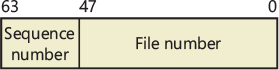
Figure 11-33 File record number.

File records

Instead of viewing a file as just a repository for textual or binary data, NTFS stores files as a collection of attribute/value pairs, one of which is the data it contains (called the unnamed data attribute). Other attributes that compose a file include the file name, time stamp information, and possibly additional named data attributes. Figure 11-34 illustrates an MFT record for a small file.

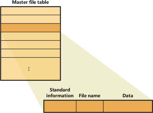
Figure 11-34 MFT record for a small file.

Each file attribute is stored as a separate stream of bytes within a file. Strictly speaking, NTFS doesn’t read and write files; it reads and writes attribute streams. NTFS supplies these attribute operations: create, delete, read (byte range), and write (byte range). The read and write services normally operate on the file’s unnamed data attribute. However, a caller can specify a different data attribute by using the named data stream syntax.

Table 11-6 lists the attributes for files on an NTFS volume. (Not all attributes are present for every file.) Each attribute in the NTFS file system can be unnamed or can have a name. An example of a named attribute is the $LOGGED_UTILITY_STREAM, which is used for various purposes by different NTFS components. Table 11-7 lists the possible $LOGGED_UTILITY_STREAM attribute’s names and their respective purposes.

Table 11-6 Attributes for NTFS files

Attribute	Attribute Type Name	Resident?	Description
Volume information	$VOLUME_INFORMATION, $VOLUME_NAME	Always, Always	These attributes are present only in the $Volume metadata file. They store volume version and label information.
Standard information	$STANDARD_INFORMATION	Always	File attributes such as read-only, archive, and so on; time stamps, including when the file was created or last modified.
File name	$FILE_NAME	Maybe	The file’s name in Unicode 1.0 characters. A file can have multiple file name attributes, as it does when a hard link to a file exists or when a file with a long name has an automatically generated short name for access by MS-DOS and 16-bit Windows applications.
Security descriptor	$SECURITY_DESCRIPTOR	Maybe	This attribute is present for backward compatibility with previous versions of NTFS and is rarely used in the current version of NTFS (3.1). NTFS stores almost all security descriptors in the $Secure metadata file, sharing descriptors among files and directories that have the same settings. Previous versions of NTFS stored private security descriptor information with each file and directory. Some files still include a $SECURITY_DESCRIPTOR attribute, such as $Boot.
Data	$DATA	Maybe	The contents of the file. In NTFS, a file has one default unnamed data attribute and can have additional named data attributes—that is, a file can have multiple data streams. A directory has no default data attribute but can have optional named data attributes. Named data streams can be used even for particular system purposes. For example, the Storage Reserve Area Table (SRAT) stream ($SRAT) is used by the Storage Service for creating Space reservations on a volume. This attribute is applied only on the $Bitmap metadata file. Storage Reserves are described later in this chapter.
Index root, index allocation	$INDEX_ROOT, $INDEX_ALLOCATION,	Always, Never	Three attributes used to implement B-tree data structures used by directories, security, quota, and other metadata files.
Attribute list	$ATTRIBUTE_LIST	Maybe	A list of the attributes that make up the file and the file record number of the MFT entry where each attribute is located. This attribute is present when a file requires more than one MFT file record.
Index Bitmap	$BITMAP	Maybe	This attribute is used for different purposes: for nonresident directories (where an $INDEX_ ALLOCATION always exists), the bitmap records which 4 KB-sized index blocks are already in use by the B-tree, and which are free for future use as B-tree grows; In the MFT there is an unnamed “$Bitmap” attribute that tracks which MFT segments are in use, and which are free for future use by new files or by existing files that require more space.
Object ID	$OBJECT_ID	Always	A 16-byte identifier (GUID) for a file or directory. The link-tracking service assigns object IDs to shell shortcut and OLE link source files. NTFS provides APIs so that files and directories can be opened with their object ID rather than their file name.
Reparse information	$REPARSE_POINT	Maybe	This attribute stores a file’s reparse point data. NTFS junctions and mount points include this attribute.
Extended attributes	$EA, $EA_INFORMATION	Maybe, Always	Extended attributes are name/value pairs and aren’t normally used but are provided for backward compatibility with OS/2 applications.
Logged utility stream	$LOGGED_UTILITY_STREAM	Maybe	This attribute type can be used for various purposes by different NTFS components. See Table 11-7 for more details.

Table 11-7 $LOGGED_UTILITY_STREAM attribute

Attribute	Attribute Type Name	Resident?	Description
Encrypted File Stream	$EFS	Maybe	EFS stores data in this attribute that’s used to manage a file’s encryption, such as the encrypted version of the key needed to decrypt the file and a list of users who are authorized to access the file.
Online encryption backup	$EfsBackup	Maybe	The attribute is used by the EFS Online encryption to store chunks of the original encrypted data stream.
Transactional NTFSData	$TXF_DATA	Maybe	When a file or directory becomes part of a transaction, TxF also stores transaction data in the $TXF_DATA attribute, such as the file’s unique transaction ID.
Desired Storage Class	$DSC	Resident	The desired storage class is used for “pinning” a file to a preferred storage tier. See the “NTFS support for tiered volumes” section for more details.

Table 11-6 shows attribute names; however, attributes actually correspond to numeric type codes, which NTFS uses to order the attributes within a file record. The file attributes in an MFT record are ordered by these type codes (numerically in ascending order), with some attribute types appearing more than once—if a file has multiple data attributes, for example, or multiple file names. All possible attribute types (and their names) are listed in the $AttrDef metadata file.

Each attribute in a file record is identified with its attribute type code and has a value and an optional name. An attribute’s value is the byte stream composing the attribute. For example, the value of the $FILE_NAME attribute is the file’s name; the value of the $DATA attribute is whatever bytes the user stored in the file.

Most attributes never have names, although the index-related attributes and the $DATA attribute often do. Names distinguish between multiple attributes of the same type that a file can include. For example, a file that has a named data stream has two $DATA attributes: an unnamed $DATA attribute storing the default unnamed data stream, and a named $DATA attribute having the name of the alternate stream and storing the named stream’s data.

File names

Both NTFS and FAT allow each file name in a path to be as many as 255 characters long. File names can contain Unicode characters as well as multiple periods and embedded spaces. However, the FAT file system supplied with MS-DOS is limited to 8 (non-Unicode) characters for its file names, followed by a period and a 3-character extension. Figure 11-35 provides a visual representation of the different file namespaces Windows supports and shows how they intersect.

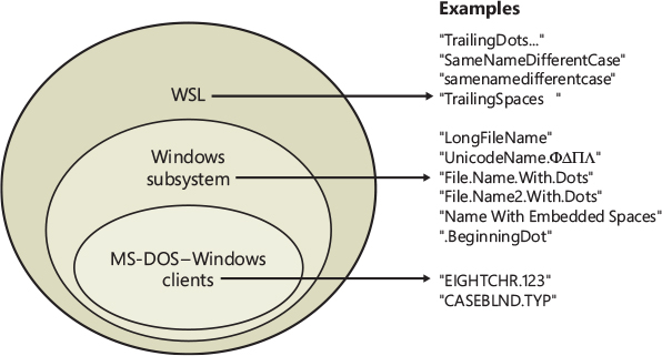
Figure 11-35 Windows file namespaces.

Windows Subsystem for Linux (WSL) requires the biggest namespace of all the application execution environments that Windows supports, and therefore the NTFS namespace is equivalent to the WSL namespace. WSL can create names that aren’t visible to Windows and MS-DOS applications, including names with trailing periods and trailing spaces. Ordinarily, creating a file using the large POSIX namespace isn’t a problem because you would do that only if you intended WSL applications to use that file.

The relationship between 32-bit Windows applications and MS-DOS and 16-bit Windows applications is a much closer one, however. The Windows area in Figure 11-35 represents file names that the Windows subsystem can create on an NTFS volume but that MS-DOS and 16-bit Windows applications can’t see. This group includes file names longer than the 8.3 format of MS-DOS names, those containing Unicode (international) characters, those with multiple period characters or a beginning period, and those with embedded spaces. For compatibility reasons, when a file is created with such a name, NTFS automatically generates an alternate, MS-DOS-style file name for the file. Windows displays these short names when you use the /x option with the dir command.

The MS-DOS file names are fully functional aliases for the NTFS files and are stored in the same directory as the long file names. The MFT record for a file with an autogenerated MS-DOS file name is shown in Figure 11-36.

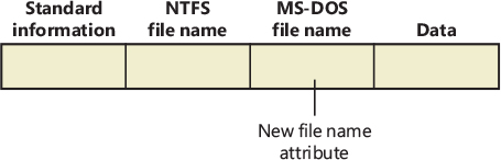
Figure 11-36 MFT file record with an MS-DOS file name attribute.

The NTFS name and the generated MS-DOS name are stored in the same file record and therefore refer to the same file. The MS-DOS name can be used to open, read from, write to, or copy the file. If a user renames the file using either the long file name or the short file name, the new name replaces both the existing names. If the new name isn’t a valid MS-DOS name, NTFS generates another MS-DOS name for the file. (Note that NTFS only generates MS-DOS-style file names for the first file name.)

Note

Hard links are implemented in a similar way. When a hard link to a file is created, NTFS adds another file name attribute to the file’s MFT file record, and adds an entry in the Index Allocation attribute of the directory in which the new link resides. The two situations differ in one regard, however. When a user deletes a file that has multiple names (hard links), the file record and the file remain in place. The file and its record are deleted only when the last file name (hard link) is deleted. If a file has both an NTFS name and an autogenerated MS-DOS name, however, a user can delete the file using either name.

Here’s the algorithm NTFS uses to generate an MS-DOS name from a long file name. The algorithm is actually implemented in the kernel function RtlGenerate8dot3Name and can change in future Windows releases. The latter function is also used by other drivers, such as CDFS, FAT, and third-party file systems:

1. Remove from the long name any characters that are illegal in MS-DOS names, including spaces and Unicode characters. Remove preceding and trailing periods. Remove all other embedded periods, except the last one.

2. Truncate the string before the period (if present) to six characters (it may already be six or fewer because this algorithm is applied when any character that is illegal in MS-DOS is present in the name). If it is two or fewer characters, generate and concatenate a four-character hex checksum string. Append the string ~n (where n is a number, starting with 1, that is used to distinguish different files that truncate to the same name). Truncate the string after the period (if present) to three characters.

3. Put the result in uppercase letters. MS-DOS is case-insensitive, and this step guarantees that NTFS won’t generate a new name that differs from the old name only in case.

4. If the generated name duplicates an existing name in the directory, increment the ~n string. If n is greater than 4, and a checksum was not concatenated already, truncate the string before the period to two characters and generate and concatenate a four-character hex checksum string.

Table 11-8 shows the long Windows file names from Figure 11-35 and their NTFS-generated MS-DOS versions. The current algorithm and the examples in Figure 11-35 should give you an idea of what NTFS-generated MS-DOS-style file names look like.

Table 11-8 NTFS-generated file names

Windows Long Name	NTFS-Generated Short Name
LongFileName	LONGFI~1
UnicodeName.FDPL	UNICOD~1
File.Name.With.Dots	FILENA~1.DOT
File.Name2.With.Dots	FILENA~2.DOT
File.Name3.With.Dots	FILENA~3.DOT
File.Name4.With.Dots	FILENA~4.DOT
File.Name5.With.Dots	FIF596~1.DOT
Name With Embedded Spaces	NAMEWI~1
.BeginningDot	BEGINN~1
25¢.two characters	255440~1.TWO
©	6E2D~1

Note

Since Windows 8.1, by default all the NTFS nonbootable volumes have short name generation disabled. You can disable short name generation even in older version of Windows by setting HKLM\SYSTEM\CurrentControlSet\Control\FileSystem\NtfsDisable8dot3NameCreation in the registry to a DWORD value of 1 and restarting the machine. This could potentially break compatibility with older applications, though.

Tunneling

NTFS uses the concept of tunneling to allow compatibility with older programs that depend on the file system to cache certain file metadata for a period of time even after the file is gone, such as when it has been deleted or renamed. With tunneling, any new file created with the same name as the original file, and within a certain period of time, will keep some of the same metadata. The idea is to replicate behavior expected by MS-DOS programs when using the safe save programming method, in which modified data is copied to a temporary file, the original file is deleted, and then the temporary file is renamed to the original name. The expected behavior in this case is that the renamed temporary file should appear to be the same as the original file; otherwise, the creation time would continuously update itself with each modification (which is how the modified time is used).

NTFS uses tunneling so that when a file name is removed from a directory, its long name and short name, as well as its creation time, are saved into a cache. When a new file is added to a directory, the cache is searched to see whether there is any tunneled data to restore. Because these operations apply to directories, each directory instance has its own cache, which is deleted if the directory is removed. NTFS will use tunneling for the following series of operations if the names used result in the deletion and re-creation of the same file name:

• ■    Delete + Create

• ■    Delete + Rename

• ■    Rename + Create

• ■    Rename + Rename

By default, NTFS keeps the tunneling cache for 15 seconds, although you can modify this timeout by creating a new value called MaximumTunnelEntryAgeInSeconds in the HKLM\SYSTEM\CurrentControlSet\Control\FileSystem registry key. Tunneling can also be completely disabled by creating a new value called MaximumTunnelEntries and setting it to 0; however, this will cause older applications to break if they rely on the compatibility behavior. On NTFS volumes that have short name generation disabled (see the previous section), tunneling is disabled by default.

You can see tunneling in action with the following simple experiment in the command prompt:

1. Create a file called file1.

2. Wait for more than 15 seconds (the default tunnel cache timeout).

3. Create a file called file2.

4. Perform a dir /TC. Note the creation times.

5. Rename file1 to file.

6. Rename file2 to file1.

7. Perform a dir /TC. Note that the creation times are identical.

Resident and nonresident attributes

If a file is small, all its attributes and their values (its data, for example) fit within the file record that describes the file. When the value of an attribute is stored in the MFT (either in the file’s main file record or an extension record located elsewhere within the MFT), the attribute is called a resident attribute. (In Figure 11-37, for example, all attributes are resident.) Several attributes are defined as always being resident so that NTFS can locate nonresident attributes. The standard information and index root attributes are always resident, for example.

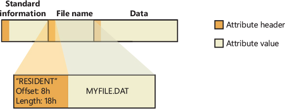
Figure 11-37 Resident attribute header and value.

Each attribute begins with a standard header containing information about the attribute—information that NTFS uses to manage the attributes in a generic way. The header, which is always resident, records whether the attribute’s value is resident or nonresident. For resident attributes, the header also contains the offset from the header to the attribute’s value and the length of the attribute’s value, as Figure 11-37 illustrates for the file name attribute.

When an attribute’s value is stored directly in the MFT, the time it takes NTFS to access the value is greatly reduced. Instead of looking up a file in a table and then reading a succession of allocation units to find the file’s data (as the FAT file system does, for example), NTFS accesses the disk once and retrieves the data immediately.

The attributes for a small directory, as well as for a small file, can be resident in the MFT, as Figure 11-38 shows. For a small directory, the index root attribute contains an index (organized as a B-tree) of file record numbers for the files (and the subdirectories) within the directory.

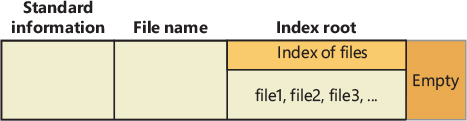
Figure 11-38 MFT file record for a small directory.

Of course, many files and directories can’t be squeezed into a 1 KB or 4 KB, fixed-size MFT record. If a particular attribute’s value, such as a file’s data attribute, is too large to be contained in an MFT file record, NTFS allocates clusters for the attribute’s value outside the MFT. A contiguous group of clusters is called a run (or an extent). If the attribute’s value later grows (if a user appends data to the file, for example), NTFS allocates another run for the additional data. Attributes whose values are stored in runs (rather than within the MFT) are called nonresident attributes. The file system decides whether a particular attribute is resident or nonresident; the location of the data is transparent to the process accessing it.

When an attribute is nonresident, as the data attribute for a large file will certainly be, its header contains the information NTFS needs to locate the attribute’s value on the disk. Figure 11-39 shows a nonresident data attribute stored in two runs.

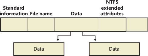
Figure 11-39 MFT file record for a large file with two data runs.

Among the standard attributes, only those that can grow can be nonresident. For files, the attributes that can grow are the data and the attribute list (not shown in Figure 11-39). The standard information and file name attributes are always resident.

A large directory can also have nonresident attributes (or parts of attributes), as Figure 11-40 shows. In this example, the MFT file record doesn’t have enough room to store the B-tree that contains the index of files that are within this large directory. A part of the index is stored in the index root attribute, and the rest of the index is stored in nonresident runs called index allocations. The index root, index allocation, and bitmap attributes are shown here in a simplified form. They are described in more detail in the next section. The standard information and file name attributes are always resident. The header and at least part of the value of the index root attribute are also resident for directories.

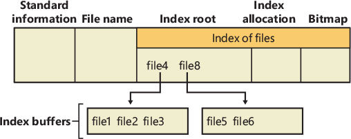
Figure 11-40 MFT file record for a large directory with a nonresident file name index.

When an attribute’s value can’t fit in an MFT file record and separate allocations are needed, NTFS keeps track of the runs by means of VCN-to-LCN mapping pairs. LCNs represent the sequence of clusters on an entire volume from 0 through n. VCNs number the clusters belonging to a particular file from 0 through m. For example, the clusters in the runs of a nonresident data attribute are numbered as shown in Figure 11-41.

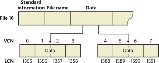
Figure 11-41 VCNs for a nonresident data attribute.

If this file had more than two runs, the numbering of the third run would start with VCN 8. As Figure 11-42 shows, the data attribute header contains VCN-to-LCN mappings for the two runs here, which allows NTFS to easily find the allocations on the disk.

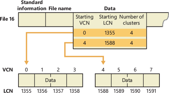
Figure 11-42 VCN-to-LCN mappings for a nonresident data attribute.

Although Figure 11-41 shows just data runs, other attributes can be stored in runs if there isn’t enough room in the MFT file record to contain them. And if a particular file has too many attributes to fit in the MFT record, a second MFT record is used to contain the additional attributes (or attribute headers for nonresident attributes). In this case, an attribute called the attribute list is added. The attribute list attribute contains the name and type code of each of the file’s attributes and the file number of the MFT record where the attribute is located. The attribute list attribute is provided for those cases where all of a file’s attributes will not fit within the file’s file record or when a file grows so large or so fragmented that a single MFT record can’t contain the multitude of VCN-to-LCN mappings needed to find all its runs. Files with more than 200 runs typically require an attribute list. In summary, attribute headers are always contained within file records in the MFT, but an attribute’s value may be located outside the MFT in one or more extents.

Data compression and sparse files

NTFS supports compression on a per-file, per-directory, or per-volume basis using a variant of the LZ77 algorithm, known as LZNT1. (NTFS compression is performed only on user data, not file system metadata.) In Windows 8.1 and later, files can also be compressed using a newer suite of algorithms, which include LZX (most compact) and XPRESS (including using 4, 8, or 16K block sizes, in order of speed). This type of compression, which can be used through commands such as the compact shell command (as well as File Provder APIs), leverages the Windows Overlay Filter (WOF) file system filter driver (Wof.sys), which uses an NTFS alternate data stream and sparse files, and is not part of the NTFS driver per se. WOF is outside the scope of this book, but you can read more about it here: https://devblogs.microsoft.com/oldnewthing/20190618-00/?p=102597.

You can tell whether a volume is compressed by using the Windows GetVolumeInformation function. To retrieve the actual compressed size of a file, use the Windows GetCompressedFileSize function. Finally, to examine or change the compression setting for a file or directory, use the Windows DeviceIoControl function. (See the FSCTL_GET_COMPRESSION and FSCTL_SET_COMPRESSION file system control codes.) Keep in mind that although setting a file’s compression state compresses (or decompresses) the file right away, setting a directory’s or volume’s compression state doesn’t cause any immediate compression or decompression. Instead, setting a directory’s or volume’s compression state sets a default compression state that will be given to all newly created files and subdirectories within that directory or volume (although, if you were to set directory compression using the directory’s property page within Explorer, the contents of the entire directory tree will be compressed immediately).

The following section introduces NTFS compression by examining the simple case of compressing sparse data. The subsequent sections extend the discussion to the compression of ordinary files and sparse files.

Note

NTFS compression is not supported in DAX volumes or for encrypted files.

Compressing sparse data

Sparse data is often large but contains only a small amount of nonzero data relative to its size. A sparse matrix is one example of sparse data. As described earlier, NTFS uses VCNs, from 0 through m, to enumerate the clusters of a file. Each VCN maps to a corresponding LCN, which identifies the disk location of the cluster. Figure 11-43 illustrates the runs (disk allocations) of a normal, noncompressed file, including its VCNs and the LCNs they map to.

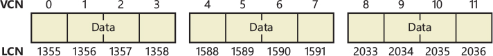
Figure 11-43 Runs of a noncompressed file.

This file is stored in three runs, each of which is 4 clusters long, for a total of 12 clusters. Figure 11-44 shows the MFT record for this file. As described earlier, to save space, the MFT record’s data attribute, which contains VCN-to-LCN mappings, records only one mapping for each run, rather than one for each cluster. Notice, however, that each VCN from 0 through 11 has a corresponding LCN associated with it. The first entry starts at VCN 0 and covers 4 clusters, the second entry starts at VCN 4 and covers 4 clusters, and so on. This entry format is typical for a noncompressed file.

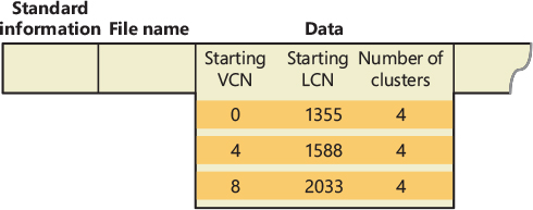
Figure 11-44 MFT record for a noncompressed file.

When a user selects a file on an NTFS volume for compression, one NTFS compression technique is to remove long strings of zeros from the file. If the file’s data is sparse, it typically shrinks to occupy a fraction of the disk space it would otherwise require. On subsequent writes to the file, NTFS allocates space only for runs that contain nonzero data.

Figure 11-45 depicts the runs of a compressed file containing sparse data. Notice that certain ranges of the file’s VCNs (16–31 and 64–127) have no disk allocations.

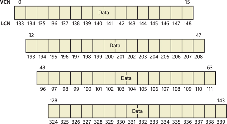
Figure 11-45 Runs of a compressed file containing sparse data.

The MFT record for this compressed file omits blocks of VCNs that contain zeros and therefore have no physical storage allocated to them. The first data entry in Figure 11-46, for example, starts at VCN 0 and covers 16 clusters. The second entry jumps to VCN 32 and covers 16 clusters.

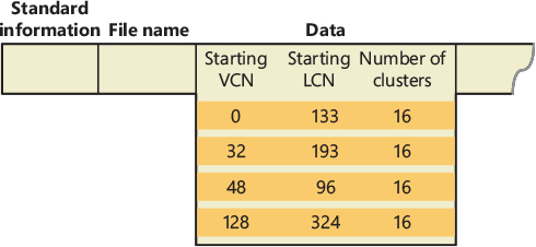
Figure 11-46 MFT record for a compressed file containing sparse data.

When a program reads data from a compressed file, NTFS checks the MFT record to determine whether a VCN-to-LCN mapping covers the location being read. If the program is reading from an unallocated “hole” in the file, it means that the data in that part of the file consists of zeros, so NTFS returns zeros without further accessing the disk. If a program writes nonzero data to a “hole,” NTFS quietly allocates disk space and then writes the data. This technique is very efficient for sparse file data that contains a lot of zero data.

Compressing nonsparse data

The preceding example of compressing a sparse file is somewhat contrived. It describes “compression” for a case in which whole sections of a file were filled with zeros, but the remaining data in the file wasn’t affected by the compression. The data in most files isn’t sparse, but it can still be compressed by the application of a compression algorithm.

In NTFS, users can specify compression for individual files or for all the files in a directory. (New files created in a directory marked for compression are automatically compressed—existing files must be compressed individually when programmatically enabling compression with FSCTL_SET_COMPRESSION.) When it compresses a file, NTFS divides the file’s unprocessed data into compression units 16 clusters long (equal to 128 KB for a 8 KB cluster, for example). Certain sequences of data in a file might not compress much, if at all; so for each compression unit in the file, NTFS determines whether compressing the unit will save at least 1 cluster of storage. If compressing the unit won’t free up at least 1 cluster, NTFS allocates a 16-cluster run and writes the data in that unit to disk without compressing it. If the data in a 16-cluster unit will compress to 15 or fewer clusters, NTFS allocates only the number of clusters needed to contain the compressed data and then writes it to disk. Figure 11-47 illustrates the compression of a file with four runs. The unshaded areas in this figure represent the actual storage locations that the file occupies after compression. The first, second, and fourth runs were compressed; the third run wasn’t. Even with one noncompressed run, compressing this file saved 26 clusters of disk space, or 41%.

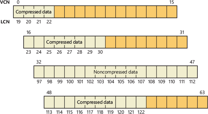
Figure 11-47 Data runs of a compressed file.

Note

Although the diagrams in this chapter show contiguous LCNs, a compression unit need not be stored in physically contiguous clusters. Runs that occupy noncontiguous clusters produce slightly more complicated MFT records than the one shown in Figure 11-47.

When it writes data to a compressed file, NTFS ensures that each run begins on a virtual 16-cluster boundary. Thus the starting VCN of each run is a multiple of 16, and the runs are no longer than 16 clusters. NTFS reads and writes at least one compression unit at a time when it accesses compressed files. When it writes compressed data, however, NTFS tries to store compression units in physically contiguous locations so that it can read them all in a single I/O operation. The 16-cluster size of the NTFS compression unit was chosen to reduce internal fragmentation: the larger the compression unit, the less the overall disk space needed to store the data. This 16-cluster compression unit size represents a trade-off between producing smaller compressed files and slowing read operations for programs that randomly access files. The equivalent of 16 clusters must be decompressed for each cache miss. (A cache miss is more likely to occur during random file access.) Figure 11-48 shows the MFT record for the compressed file shown in Figure 11-47.

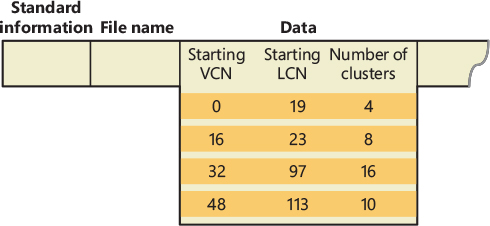
Figure 11-48 MFT record for a compressed file.

One difference between this compressed file and the earlier example of a compressed file containing sparse data is that three of the compressed runs in this file are less than 16 clusters long. Reading this information from a file’s MFT file record enables NTFS to know whether data in the file is compressed. Any run shorter than 16 clusters contains compressed data that NTFS must decompress when it first reads the data into the cache. A run that is exactly 16 clusters long doesn’t contain compressed data and therefore requires no decompression.

If the data in a run has been compressed, NTFS decompresses the data into a scratch buffer and then copies it to the caller’s buffer. NTFS also loads the decompressed data into the cache, which makes subsequent reads from the same run as fast as any other cached read. NTFS writes any updates to the file to the cache, leaving the lazy writer to compress and write the modified data to disk asynchronously. This strategy ensures that writing to a compressed file produces no more significant delay than writing to a noncompressed file would.

NTFS keeps disk allocations for a compressed file contiguous whenever possible. As the LCNs indicate, the first two runs of the compressed file shown in Figure 11-47 are physically contiguous, as are the last two. When two or more runs are contiguous, NTFS performs disk read-ahead, as it does with the data in other files. Because the reading and decompression of contiguous file data take place asynchronously before the program requests the data, subsequent read operations obtain the data directly from the cache, which greatly enhances read performance.

Sparse files

Sparse files (the NTFS file type, as opposed to files that consist of sparse data, as described earlier) are essentially compressed files for which NTFS doesn’t apply compression to the file’s nonsparse data. However, NTFS manages the run data of a sparse file’s MFT record the same way it does for compressed files that consist of sparse and nonsparse data.

The change journal file

The change journal file, \$Extend\$UsnJrnl, is a sparse file in which NTFS stores records of changes to files and directories. Applications like the Windows File Replication Service (FRS) and the Windows Search service make use of the journal to respond to file and directory changes as they occur.

The journal stores change entries in the $J data stream and the maximum size of the journal in the $Max data stream. Entries are versioned and include the following information about a file or directory change:

• ■    The time of the change

• ■    The reason for the change (see Table 11-9)

• ■    The file or directory’s attributes

• ■    The file or directory’s name

• ■    The file or directory’s MFT file record number

• ■    The file record number of the file’s parent directory

• ■    The security ID

• ■    The update sequence number (USN) of the record

• ■    Additional information about the source of the change (a user, the FRS, and so on)

Table 11-9 Change journal change reasons

Identifier	Reason
USN_REASON_DATA_OVERWRITE	The data in the file or directory was overwritten.
USN_REASON_DATA_EXTEND	Data was added to the file or directory.
USN_REASON_DATA_TRUNCATION	The data in the file or directory was truncated.
USN_REASON_NAMED_DATA_OVERWRITE	The data in a file’s data stream was overwritten.
USN_REASON_NAMED_DATA_EXTEND	The data in a file’s data stream was extended.
USN_REASON_NAMED_DATA_TRUNCATION	The data in a file’s data stream was truncated.
USN_REASON_FILE_CREATE	A new file or directory was created.
USN_REASON_FILE_DELETE	A file or directory was deleted.
USN_REASON_EA_CHANGE	The extended attributes for a file or directory changed.
USN_REASON_SECURITY_CHANGE	The security descriptor for a file or directory was changed.
USN_REASON_RENAME_OLD_NAME	A file or directory was renamed; this is the old name.
USN_REASON_RENAME_NEW_NAME	A file or directory was renamed; this is the new name.
USN_REASON_INDEXABLE_CHANGE	The indexing state for the file or directory was changed (whether or not the Indexing service will process this file or directory).
USN_REASON_BASIC_INFO_CHANGE	The file or directory attributes and/or the time stamps were changed.
USN_REASON_HARD_LINK_CHANGE	A hard link was added or removed from the file or directory.
USN_REASON_COMPRESSION_CHANGE	The compression state for the file or directory was changed.
USN_REASON_ENCRYPTION_CHANGE	The encryption state (EFS) was enabled or disabled for this file or directory.
USN_REASON_OBJECT_ID_CHANGE	The object ID for this file or directory was changed.
USN_REASON_REPARSE_POINT_CHANGE	The reparse point for a file or directory was changed, or a new reparse point (such as a symbolic link) was added or deleted from a file or directory.
USN_REASON_STREAM_CHANGE	A new data stream was added to or removed from a file or renamed.
USN_REASON_TRANSACTED_CHANGE	This value is added (ORed) to the change reason to indicate that the change was the result of a recent commit of a TxF transaction.
USN_REASON_CLOSE	The handle to a file or directory was closed, indicating that this is the final modification made to the file in this series of operations.
USN_REASON_INTEGRITY_CHANGE	The content of a file’s extent (run) has changed, so the associated integrity stream has been updated with a new checksum. This Identifier is generated by the ReFS file system.
USN_REASON_DESIRED_STORAGE_CLASS_CHANGE	The event is generated by the NTFS file system driver when a stream is moved from the capacity to the performance tier or vice versa.

EXPERIMENT: Reading the change journal

You can use the built-in %SystemRoot%\System32\Fsutil.exe tool to create, delete, or query journal information with the built-in Fsutil.exe utility, as shown here:

Click here to view code image

d:\>fsutil usn queryjournal d:
    Usn Journal ID   : 0x01d48f4c3853cc72
    First Usn        : 0x0000000000000000
    Next Usn         : 0x0000000000000a60
    Lowest Valid Usn : 0x0000000000000000
    Max Usn          : 0x7fffffffffff0000
    Maximum Size     : 0x0000000000a00000
    Allocation Delta : 0x0000000000200000
    Minimum record version supported : 2
    Maximum record version supported : 4
    Write range tracking: Disabled

The output indicates the maximum size of the change journal on the volume (10 MB) and its current state. As a simple experiment to see how NTFS records changes in the journal, create a file called Usn.txt in the current directory, rename it to UsnNew.txt, and then dump the journal with Fsutil, as shown here:

Click here to view code image

d:\>echo Hello USN Journal! > Usn.txt
    d:\>ren Usn.txt UsnNew.txt
    d:\>fsutil usn readjournal d:
    ...
    
    Usn               : 2656
    File name         : Usn.txt
    File name length  : 14
    Reason            : 0x00000100: File create
    Time stamp        : 12/8/2018 15:22:05
    File attributes   : 0x00000020: Archive
    File ID           : 0000000000000000000c000000617912
    Parent file ID    : 00000000000000000018000000617ab6
    Source info       : 0x00000000: *NONE*
    Security ID       : 0
    Major version     : 3
    Minor version     : 0
    Record length     : 96
    
    Usn               : 2736
    File name         : Usn.txt
    File name length  : 14
    Reason            : 0x00000102: Data extend | File create
    Time stamp        : 12/8/2018 15:22:05
    File attributes   : 0x00000020: Archive
    File ID           : 0000000000000000000c000000617912
    Parent file ID    : 00000000000000000018000000617ab6
    Source info       : 0x00000000: *NONE*
    Security ID       : 0
    Major version     : 3
    Minor version     : 0
    Record length     : 96
    
    Usn               : 2816
    File name         : Usn.txt
    File name length  : 14
    Reason            : 0x80000102: Data extend | File create | Close
    Time stamp        : 12/8/2018 15:22:05
    File attributes   : 0x00000020: Archive
    File ID           : 0000000000000000000c000000617912
    Parent file ID    : 00000000000000000018000000617ab6
    Source info       : 0x00000000: *NONE*
    Security ID       : 0
    Major version     : 3
    Minor version     : 0
    Record length     : 96
    
    Usn               : 2896
    File name         : Usn.txt
    File name length  : 14
    Reason            : 0x00001000: Rename: old name
    Time stamp        : 12/8/2018 15:22:15
    File attributes   : 0x00000020: Archive
    File ID           : 0000000000000000000c000000617912
    Parent file ID    : 00000000000000000018000000617ab6
    Source info       : 0x00000000: *NONE*
    Security ID       : 0
    Major version     : 3
    Minor version     : 0
    Record length     : 96
    
    Usn               : 2976
    File name         : UsnNew.txt
    File name length  : 20
    Reason            : 0x00002000: Rename: new name
    Time stamp        : 12/8/2018 15:22:15
    File attributes   : 0x00000020: Archive
    File ID           : 0000000000000000000c000000617912
    Parent file ID    : 00000000000000000018000000617ab6
    Source info       : 0x00000000: *NONE*
    Security ID       : 0
    Major version     : 3
    Minor version     : 0
    Record length     : 96
    
    Usn               : 3056
    File name         : UsnNew.txt
    File name length  : 20
    Reason            : 0x80002000: Rename: new name | Close
    Time stamp        : 12/8/2018 15:22:15
    File attributes   : 0x00000020: Archive
    File ID           : 0000000000000000000c000000617912
    Parent file ID    : 00000000000000000018000000617ab6
    Source info       : 0x00000000: *NONE*
    Security ID       : 0
    Major version     : 3
    Minor version     : 0
    Record length     : 96

The entries reflect the individual modification operations involved in the operations underlying the command-line operations. If the change journal isn’t enabled on a volume (this happens especially on non-system volumes where no applications have requested file change notification or the USN Journal creation), you can easily create it with the following command (in the example a 10-MB journal has been requested):

Click here to view code image

d:\ >fsutil usn createJournal d: m=10485760 a=2097152

The journal is sparse so that it never overflows; when the journal’s on-disk size exceeds the maximum defined for the file, NTFS simply begins zeroing the file data that precedes the window of change information having a size equal to the maximum journal size, as shown in Figure 11-49. To prevent constant resizing when an application is continuously exceeding the journal’s size, NTFS shrinks the journal only when its size is twice an application-defined value over the maximum configured size.

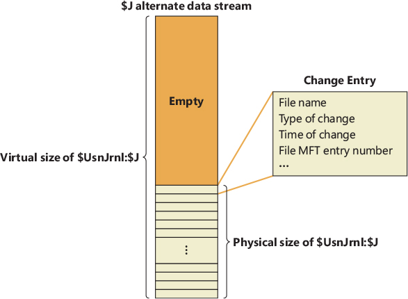
Figure 11-49 Change journal ($UsnJrnl) space allocation.

Indexing

In NTFS, a file directory is simply an index of file names—that is, a collection of file names (along with their file record numbers) organized as a B-tree. To create a directory, NTFS indexes the file name attributes of the files in the directory. The MFT record for the root directory of a volume is shown in Figure 11-50.

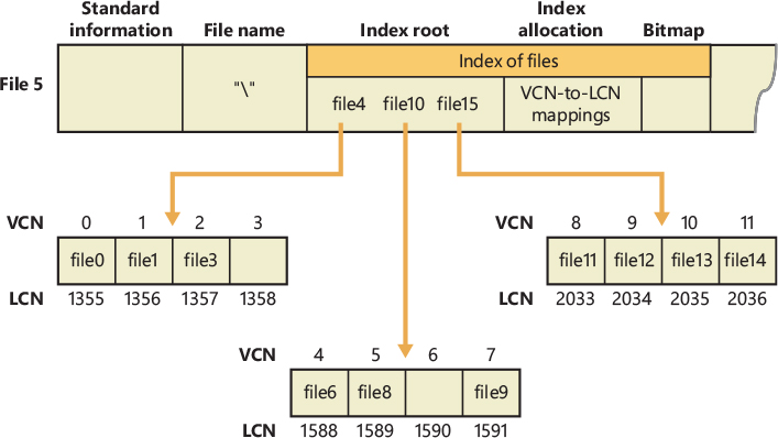
Figure 11-50 File name index for a volume’s root directory.

Conceptually, an MFT entry for a directory contains in its index root attribute a sorted list of the files in the directory. For large directories, however, the file names are actually stored in 4 KB, fixed-size index buffers (which are the nonresident values of the index allocation attribute) that contain and organize the file names. Index buffers implement a B-tree data structure, which minimizes the number of disk accesses needed to find a particular file, especially for large directories. The index root attribute contains the first level of the B-tree (root subdirectories) and points to index buffers containing the next level (more subdirectories, perhaps, or files).

Figure 11-50 shows only file names in the index root attribute and the index buffers (file6, for example), but each entry in an index also contains the record number in the MFT where the file is described and time stamp and file size information for the file. NTFS duplicates the time stamps and file size information from the file’s MFT record. This technique, which is used by FAT and NTFS, requires updated information to be written in two places. Even so, it’s a significant speed optimization for directory browsing because it enables the file system to display each file’s time stamps and size without opening every file in the directory.

The index allocation attribute maps the VCNs of the index buffer runs to the LCNs that indicate where the index buffers reside on the disk, and the bitmap attribute keeps track of which VCNs in the index buffers are in use and which are free. Figure 11-50 shows one file entry per VCN (that is, per cluster), but file name entries are actually packed into each cluster. Each 4 KB index buffer will typically contain about 20 to 30 file name entries (depending on the lengths of the file names within the directory).

The B-tree data structure is a type of balanced tree that is ideal for organizing sorted data stored on a disk because it minimizes the number of disk accesses needed to find an entry. In the MFT, a directory’s index root attribute contains several file names that act as indexes into the second level of the B-tree. Each file name in the index root attribute has an optional pointer associated with it that points to an index buffer. The index buffer points to containing file names with lexicographic values less than its own. In Figure 11-50, for example, file4 is a first-level entry in the B-tree. It points to an index buffer containing file names that are (lexicographically) less than itself—the file names file0, file1, and file3. Note that the names file1, file3, and so on that are used in this example are not literal file names but names intended to show the relative placement of files that are lexicographically ordered according to the displayed sequence.

Storing the file names in B-trees provides several benefits. Directory lookups are fast because the file names are stored in a sorted order. And when higher-level software enumerates the files in a directory, NTFS returns already-sorted names. Finally, because B-trees tend to grow wide rather than deep, NTFS’s fast lookup times don’t degrade as directories grow.

NTFS also provides general support for indexing data besides file names, and several NTFS features—including object IDs, quota tracking, and consolidated security—use indexing to manage internal data.

The B-tree indexes are a generic capability of NTFS and are used for organizing security descriptors, security IDs, object IDs, disk quota records, and reparse points. Directories are referred to as file name indexes, whereas other types of indexes are known as view indexes.

Object IDs

In addition to storing the object ID assigned to a file or directory in the $OBJECT_ID attribute of its MFT record, NTFS also keeps the correspondence between object IDs and their file record numbers in the $O index of the \$Extend\$ObjId metadata file. The index collates entries by object ID (which is a GUID), making it easy for NTFS to quickly locate a file based on its ID. This feature allows applications, using the NtCreateFile native API with the FILE_OPEN_BY_FILE_ID flag, to open a file or directory using its object ID. Figure 11-51 demonstrates the correspondence of the $ObjId metadata file and $OBJECT_ID attributes in MFT records.

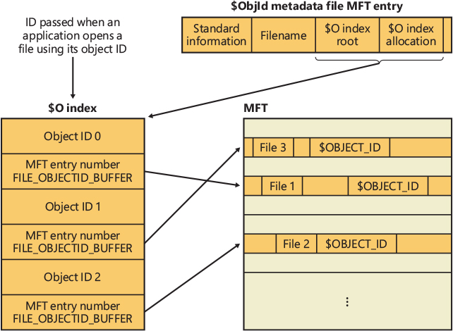
Figure 11-51 $ObjId and $OBJECT_ID relationships.

Quota tracking

NTFS stores quota information in the \$Extend\$Quota metadata file, which consists of the named index root attributes $O and $Q. Figure 11-52 shows the organization of these indexes. Just as NTFS assigns each security descriptor a unique internal security ID, NTFS assigns each user a unique user ID. When an administrator defines quota information for a user, NTFS allocates a user ID that corresponds to the user’s SID. In the $O index, NTFS creates an entry that maps an SID to a user ID and sorts the index by SID; in the $Q index, NTFS creates a quota control entry. A quota control entry contains the value of the user’s quota limits, as well as the amount of disk space the user consumes on the volume.

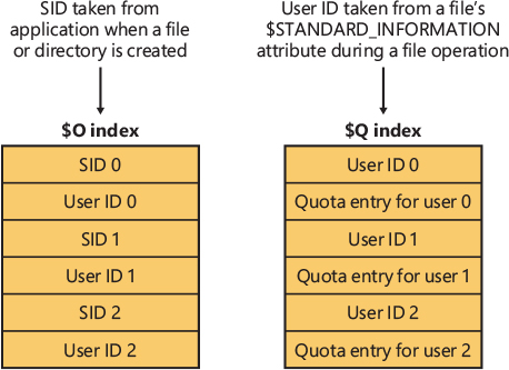
Figure 11-52 $Quota indexing.

When an application creates a file or directory, NTFS obtains the application user’s SID and looks up the associated user ID in the $O index. NTFS records the user ID in the new file or directory’s $STANDARD_INFORMATION attribute, which counts all disk space allocated to the file or directory against that user’s quota. Then NTFS looks up the quota entry in the $Q index and determines whether the new allocation causes the user to exceed his or her warning or limit threshold. When a new allocation causes the user to exceed a threshold, NTFS takes appropriate steps, such as logging an event to the System event log or not letting the user create the file or directory. As a file or directory changes size, NTFS updates the quota control entry associated with the user ID stored in the $STANDARD_INFORMATION attribute. NTFS uses the NTFS generic B-tree indexing to efficiently correlate user IDs with account SIDs and, given a user ID, to efficiently look up a user’s quota control information.

Consolidated security

NTFS has always supported security, which lets an administrator specify which users can and can’t access individual files and directories. NTFS optimizes disk utilization for security descriptors by using a central metadata file named $Secure to store only one instance of each security descriptor on a volume.

The $Secure file contains two index attributes—$SDH (Security Descriptor Hash) and $SII (Security ID Index)—and a data-stream attribute named $SDS (Security Descriptor Stream), as Figure 11-53 shows. NTFS assigns every unique security descriptor on a volume an internal NTFS security ID (not to be confused with a Windows SID, which uniquely identifies computers and user accounts) and hashes the security descriptor according to a simple hash algorithm. A hash is a potentially nonunique shorthand representation of a descriptor. Entries in the $SDH index map the security descriptor hashes to the security descriptor’s storage location within the $SDS data attribute, and the $SII index entries map NTFS security IDs to the security descriptor’s location in the $SDS data attribute.

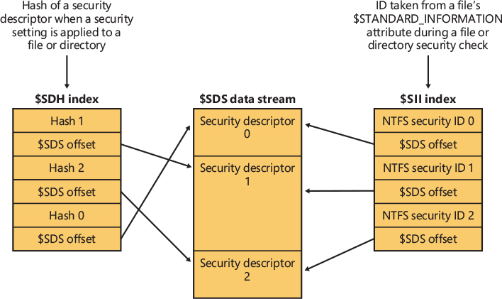
Figure 11-53 $Secure indexing.

When you apply a security descriptor to a file or directory, NTFS obtains a hash of the descriptor and looks through the $SDH index for a match. NTFS sorts the $SDH index entries according to the hash of their corresponding security descriptor and stores the entries in a B-tree. If NTFS finds a match for the descriptor in the $SDH index, NTFS locates the offset of the entry’s security descriptor from the entry’s offset value and reads the security descriptor from the $SDS attribute. If the hashes match but the security descriptors don’t, NTFS looks for another matching entry in the $SDH index. When NTFS finds a precise match, the file or directory to which you’re applying the security descriptor can reference the existing security descriptor in the $SDS attribute. NTFS makes the reference by reading the NTFS security identifier from the $SDH entry and storing it in the file or directory’s $STANDARD_INFORMATION attribute. The NTFS $STANDARD_INFORMATION attribute, which all files and directories have, stores basic information about a file, including its attributes, time stamp information, and security identifier.

If NTFS doesn’t find in the $SDH index an entry that has a security descriptor that matches the descriptor you’re applying, the descriptor you’re applying is unique to the volume, and NTFS assigns the descriptor a new internal security ID. NTFS internal security IDs are 32-bit values, whereas SIDs are typically several times larger, so representing SIDs with NTFS security IDs saves space in the $STANDARD_INFORMATION attribute. NTFS then adds the security descriptor to the end of the $SDS data attribute, and it adds to the $SDH and $SII indexes entries that reference the descriptor’s offset in the $SDS data.

When an application attempts to open a file or directory, NTFS uses the $SII index to look up the file or directory’s security descriptor. NTFS reads the file or directory’s internal security ID from the MFT entry’s $STANDARD_INFORMATION attribute. It then uses the $Secure file’s $SII index to locate the ID’s entry in the $SDS data attribute. The offset into the $SDS attribute lets NTFS read the security descriptor and complete the security check. NTFS stores the 32 most recently accessed security descriptors with their $SII index entries in a cache so that it accesses the $Secure file only when the $SII isn’t cached.

NTFS doesn’t delete entries in the $Secure file, even if no file or directory on a volume references the entry. Not deleting these entries doesn’t significantly decrease disk space because most volumes, even those used for long periods, have relatively few unique security descriptors.

NTFS’s use of generic B-tree indexing lets files and directories that have the same security settings efficiently share security descriptors. The $SII index lets NTFS quickly look up a security descriptor in the $Secure file while performing security checks, and the $SDH index lets NTFS quickly determine whether a security descriptor being applied to a file or directory is already stored in the $Secure file and can be shared.

Reparse points

As described earlier in the chapter, a reparse point is a block of up to 16 KB of application-defined reparse data and a 32-bit reparse tag that are stored in the $REPARSE_POINT attribute of a file or directory. Whenever an application creates or deletes a reparse point, NTFS updates the \$Extend\$Reparse metadata file, in which NTFS stores entries that identify the file record numbers of files and directories that contain reparse points. Storing the records in a central location enables NTFS to provide interfaces for applications to enumerate all a volume’s reparse points or just specific types of reparse points, such as mount points. The \$Extend\$Reparse file uses the generic B-tree indexing facility of NTFS by collating the file’s entries (in an index named $R) by reparse point tags and file record numbers.

EXPERIMENT: Looking at different reparse points

A file or directory reparse point can contain any kind of arbitrary data. In this experiment, we use the built-in fsutil.exe tool to analyze the reparse point content of a symbolic link and of a Modern application’s AppExecutionAlias, similar to the experiment in Chapter 8. First you need to create a symbolic link:

Click here to view code image

C:\>mklink test_link.txt d:\Test.txt
    symbolic link created for test_link.txt <<===>> d:\Test.txt

Then you can use the fsutil reparsePoint query command to examine the reparse point content:

Click here to view code image

C:\>fsutil reparsePoint query test_link.txt
    Reparse Tag Value : 0xa000000c
    Tag value: Microsoft
    Tag value: Name Surrogate
    Tag value: Symbolic Link
    
    Reparse Data Length: 0x00000040
    Reparse Data:
    0000:  16 00 1e 00 00 00 16 00  00 00 00 00 64 00 3a 00  ............d.:.
    0010:  5c 00 54 00 65 00 73 00  74 00 2e 00 74 00 78 00  \.T.e.s.t...t.x.
    0020:  74 00 5c 00 3f 00 3f 00  5c 00 64 00 3a 00 5c 00  t.\.?.?.\.d.:.\.
    0030:  54 00 65 00 73 00 74 00  2e 00 74 00 78 00 74 00  T.e.s.t...t.x.t.

As expected, the content is a simple data structure (REPARSE_DATA_BUFFER, documented in Microsoft Docs), which contains the symbolic link target and the printed file name. You can even delete the reparse point by using fsutil reparsePoint delete command:

Click here to view code image

C:\>more test_link.txt
    This is a test file!
    
    C:\>fsutil reparsePoint delete test_link.txt
    
    C:\>more test_link.txt

If you delete the reparse point, the file become a 0 bytes file. This is by design because the unnamed data stream ($DATA) in the link file is empty. You can repeat the experiment with an AppExecutionAlias of an installed Modern application (in the following example, Spotify was used):

Click here to view code image

C:\>cd C:\Users\Andrea\AppData\Local\Microsoft\WindowsApps
    C:\Users\andrea\AppData\Local\Microsoft\WindowsApps>fsutil reparsePoint query Spotify.exe
    Reparse Tag Value : 0x8000001b
    Tag value: Microsoft
    
    Reparse Data Length: 0x00000178
    Reparse Data:
    0000:  03 00 00 00 53 00 70 00  6f 00 74 00 69 00 66 00  ....S.p.o.t.i.f.
    0010:  79 00 41 00 42 00 2e 00  53 00 70 00 6f 00 74 00  y.A.B...S.p.o.t.
    0020:  69 00 66 00 79 00 4d 00  75 00 73 00 69 00 63 00  i.f.y.M.u.s.i.c.
    0030:  5f 00 7a 00 70 00 64 00  6e 00 65 00 6b 00 64 00  _.z.p.d.n.e.k.d.
    0040:  72 00 7a 00 72 00 65 00  61 00 30 00 00 00 53 00  r.z.r.e.a.0...S
    0050:  70 00 6f 00 74 00 69 00  66 00 79 00 41 00 42 00  p.o.t.i.f.y.A.B.
    0060:  2e 00 53 00 70 00 6f 00  74 00 69 00 66 00 79 00  ..S.p.o.t.i.f.y.
    0070:  4d 00 75 00 73 00 69 00  63 00 5f 00 7a 00 70 00  M.u.s.i.c._.z.p.
    0080:  64 00 6e 00 65 00 6b 00  64 00 72 00 7a 00 72 00  d.n.e.k.d.r.z.r.
    0090:  65 00 61 00 30 00 21 00  53 00 70 00 6f 00 74 00  e.a.0.!.S.p.o.t.
    00a0:  69 00 66 00 79 00 00 00  43 00 3a 00 5c 00 50 00  i.f.y...C.:.\.P.
    00b0:  72 00 6f 00 67 00 72 00  61 00 6d 00 20 00 46 00  r.o.g.r.a.m. .F.
    00c0:  69 00 6c 00 65 00 73 00  5c 00 57 00 69 00 6e 00  i.l.e.s.\.W.i.n.
    00d0:  64 00 6f 00 77 00 73 00  41 00 70 00 70 00 73 00  d.o.w.s.A.p.p.s.
    00e0:  5c 00 53 00 70 00 6f 00  74 00 69 00 66 00 79 00  \.S.p.o.t.i.f.y.
    00f0:  41 00 42 00 2e 00 53 00  70 00 6f 00 74 00 69 00  A.B...S.p.o.t.i.
    0100:  66 00 79 00 4d 00 75 00  73 00 69 00 63 00 5f 00  f.y.M.u.s.i.c._.
    0110:  31 00 2e 00 39 00 34 00  2e 00 32 00 36 00 32 00  1...9.4...2.6.2.
    0120:  2e 00 30 00 5f 00 78 00  38 00 36 00 5f 00 5f 00  ..0._.x.8.6._._.
    0130:  7a 00 70 00 64 00 6e 00  65 00 6b 00 64 00 72 00  z.p.d.n.e.k.d.r.
    0140:  7a 00 72 00 65 00 61 00  30 00 5c 00 53 00 70 00  z.r.e.a.0.\.S.p.
    0150:  6f 00 74 00 69 00 66 00  79 00 4d 00 69 00 67 00  o.t.i.f.y.M.i.g.
    0160:  72 00 61 00 74 00 6f 00  72 00 2e 00 65 00 78 00  r.a.t.o.r...e.x.
    0170:  65 00 00 00 30 00 00 00                           e...0...

From the preceding output, we can see another kind of reparse point, the AppExecutionAlias, used by Modern applications. More information is available in Chapter 8.

Storage reserves and NTFS reservations

Windows Update and the Windows Setup application must be able to correctly apply important security updates, even when the system volume is almost full (they need to ensure that there is enough disk space). Windows 10 introduced Storage Reserves as a way to achieve this goal. Before we describe the Storage Reserves, it is necessary that you understand how NTFS reservations work and why they’re needed.

When the NTFS file system mounts a volume, it calculates the volume’s in-use and free space. No on-disk attributes exist for keeping track of these two counters; NTFS maintains and stores the Volume bitmap on disk, which represents the state of all the clusters in the volume. The NTFS mounting code scans the bitmap and counts the number of used clusters, which have their bit set to 1 in the bitmap, and, through a simple equation (total number of clusters of the volume minus the number of used ones), calculates the number of free clusters. The two calculated counters are stored in the volume control block (VCB) data structure, which represents the mounted volume and exists only in memory until the volume is dismounted.

During normal volume I/O activity, NTFS must maintain the total number of reserved clusters. This counter needs to exist for the following reasons:

• ■    When writing to compressed and sparse files, the system must ensure that the entire file is writable because an application that is operating on this kind of file could potentially store valid uncompressed data on the entire file.

• ■    The first time a writable image-backed section is created, the file system must reserve available space for the entire section size, even if no physical space is still allocated in the volume.

• ■    The USN Journal and TxF use the counter to ensure that there is space available for the USN log and NTFS transactions.

NTFS maintains another counter during normal I/O activities, Total Free Available Space, which is the final space that a user can see and use for storing new files or data. These three concepts are parts of NTFS Reservations. The important characteristic of NTFS Reservations is that the counters are only in-memory volatile representations, which will be destroyed at volume dismounting time.

Storage Reserve is a feature based on NTFS reservations, which allow files to have an assigned Storage Reserve area. Storage Reserve defines 15 different reservation areas (2 of which are reserved by the OS), which are defined and stored both in memory and in the NTFS on-disk data structures.

To use the new on-disk reservations, an application defines a volume’s Storage Reserve area by using the FSCTL_QUERY_STORAGE_RESERVE file system control code, which specifies, through a data structure, the total amount of reserved space and an Area ID. This will update multiple counters in the VCB (Storage Reserve areas are maintained in-memory) and insert new data in the $SRAT named data stream of the $Bitmap metadata file. The $SRAT data stream contains a data structure that tracks each Reserve area, including the number of reserved and used clusters. An application can query information about Storage Reserve areas through the FSCTL_QUERY_STORAGE_RESERVE file system control code and can delete a Storage Reserve using the FSCTL_DELETE_STORAGE_RESERVE code.

After a Storage Reserve area is defined, the application is guaranteed that the space will no longer be used by any other components. Applications can then assign files and directories to a Storage Reserve area using the NtSetInformationFile native API with the FileStorageReserveIdInformationEx information class. The NTFS file system driver manages the request by updating the in-memory reserved and used clusters counters of the Reserve area, and by updating the volume’s total number of reserved clusters that belong to NTFS reservations. It also stores and updates the on-disk $STANDARD_INFO attribute of the target file. The latter maintains 4 bits to store the Storage Reserve area ID. In this way, the system is able to quickly enumerate each file that belongs to a reserve area by just parsing MFT entries. (NTFS implements the enumeration in the FSCTL_QUERY_FILE_LAYOUT code’s dispatch function.) A user can enumerate the files that belong to a Storage Reserve by using the fsutil storageReserve findByID command, specifying the volume path name and Storage Reserve ID she is interested in.

Several basic file operations have new side effects due to Storage Reserves, like file creation and renaming. Newly created files or directories will automatically inherit the storage reserve ID of their parent; the same applies for files or directories that get renamed (moved) to a new parent. Since a rename operation can change the Storage Reserve ID of the file or directory, this implies that the operation might fail due to lack of disk space. Moving a nonempty directory to a new parent implies that the new Storage Reserve ID is recursively applied to all the files and subdirectories. When the reserved space of a Storage Reserve ends, the system starts to use the volume’s free available space, so there is no guarantee that the operation always succeeds.

EXPERIMENT: Witnessing storage reserves

Starting from the May 2019 Update of Windows 10 (19H1), you can look at the existing NTFS reserves through the built-in fsutil.exe tool:

Click here to view code image

C:\>fsutil storagereserve query c:
    Reserve ID:       1
    Flags:            0x00000000
    Space Guarantee:  0x0               (0 MB)
    Space Used:       0x0               (0 MB)
    
    Reserve ID:       2
    Flags:            0x00000000
    Space Guarantee:  0x0               (0 MB)
    Space Used:       0x199ed000        (409 MB)

Windows Setup defines two NTFS reserves: a Hard reserve (ID 1), used by the Setup application to store its files, which can’t be deleted or replaced by other applications, and a Soft reserve (ID 2), which is used to store temporary files, like system logs and Windows Update downloaded files. In the preceding example, the Setup application has been already able to install all its files (and no Windows Update is executing), so the Hard Reserve is empty; the Soft reserve has all its reserved space allocated. You can enumerate all the files that belong to the reserve using the fsutil storagereserve findById command. (Be aware that the output is very large, so you might consider redirecting the output to a file using the > operator.)

Click here to view code image

C:\>fsutil storagereserve findbyid c: 2
    ...
    
    ********* File 0x0002000000018762 *********
    File reference number   : 0x0002000000018762
    File attributes         : 0x00000020: Archive
    File entry flags        : 0x00000000
    Link (ParentID: Name)   : 0x0001000000001165: NTFS Name    :
    Windows\System32\winevt\Logs\OAlerts.evtx
    Link (ParentID: Name)   : 0x0001000000001165: DOS Name     : OALERT~1.EVT
    Creation Time           : 12/9/2018 3:26:55
    Last Access Time        : 12/10/2018 0:21:57
    Last Write Time         : 12/10/2018 0:21:57
    Change Time             : 12/10/2018 0:21:57
    LastUsn                 : 44,846,752
    OwnerId                 : 0
    SecurityId              : 551
    StorageReserveId        : 2
    Stream                  : 0x010  ::$STANDARD_INFORMATION
        Attributes          : 0x00000000: *NONE*
        Flags               : 0x0000000c: Resident | No clusters allocated
        Size                : 72
        Allocated Size      : 72
    Stream                  : 0x030  ::$FILE_NAME
        Attributes          : 0x00000000: *NONE*
        Flags               : 0x0000000c: Resident | No clusters allocated
        Size                : 90
        Allocated Size      : 96
    Stream                  : 0x030  ::$FILE_NAME
        Attributes          : 0x00000000: *NONE*
        Flags               : 0x0000000c: Resident | No clusters allocated
        Size                : 90
        Allocated Size      : 96
    Stream                  : 0x080  ::$DATA
        Attributes          : 0x00000000: *NONE*
        Flags               : 0x00000000: *NONE*
        Size                : 69,632
        Allocated Size      : 69,632
        Extents             : 1 Extents
                            : 1: VCN: 0 Clusters: 17 LCN: 3,820,235

Transaction support

By leveraging the Kernel Transaction Manager (KTM) support in the kernel, as well as the facilities provided by the Common Log File System, NTFS implements a transactional model called transactional NTFS or TxF. TxF provides a set of user-mode APIs that applications can use for transacted operations on their files and directories and also a file system control (FSCTL) interface for managing its resource managers.

Note

Windows Vista added the support for TxF as a means to introduce atomic transactions to Windows. The NTFS driver was modified without actually changing the format of the NTFS data structures, which is why the NTFS format version number, 3.1, is the same as it has been since Windows XP and Windows Server 2003. TxF achieves backward compatibility by reusing the attribute type ($LOGGED_UTILITY_STREAM) that was previously used only for EFS support instead of adding a new one.

TxF is a powerful API, but due to its complexity and various issues that developers need to consider, they have been adopted by a low number of applications. At the time of this writing, Microsoft is considering deprecating TxF APIs in a future version of Windows. For the sake of completeness, we present only a general overview of the TxF architecture in this book.

The overall architecture for TxF, shown in Figure 11-54, uses several components:

• ■    Transacted APIs implemented in the Kernel32.dll library

• ■    A library for reading TxF logs (%SystemRoot%\System32\Txfw32.dll)

• ■    A COM component for TxF logging functionality (%SystemRoot\System32\Txflog.dll)

• ■    The transactional NTFS library inside the NTFS driver

• ■    The CLFS infrastructure for reading and writing log records

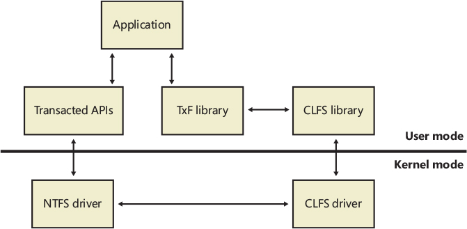
Figure 11-54 TxF architecture.

Isolation

Although transactional file operations are opt-in, just like the transactional registry (TxR) operations described in Chapter 10, TxF has an effect on regular applications that are not transaction-aware because it ensures that the transactional operations are isolated. For example, if an antivirus program is scanning a file that’s currently being modified by another application via a transacted operation, TxF must ensure that the scanner reads the pretransaction data, while applications that access the file within the transaction work with the modified data. This model is called read-committed isolation.

Read-committed isolation involves the concept of transacted writers and transacted readers. The former always view the most up-to-date version of a file, including all changes made by the transaction that is currently associated with the file. At any given time, there can be only one transacted writer for a file, which means that its write access is exclusive. Transacted readers, on the other hand, have access only to the committed version of the file at the time they open the file. They are therefore isolated from changes made by transacted writers. This allows for readers to have a consistent view of a file, even when a transacted writer commits its changes. To see the updated data, the transacted reader must open a new handle to the modified file.

Nontransacted writers, on the other hand, are prevented from opening the file by both transacted writers and transacted readers, so they cannot make changes to the file without being part of the transaction. Nontransacted readers act similarly to transacted readers in that they see only the file contents that were last committed when the file handle was open. Unlike transacted readers, however, they do not receive read-committed isolation, and as such they always receive the updated view of the latest committed version of a transacted file without having to open a new file handle. This allows non-transaction-aware applications to behave as expected.

To summarize, TxF’s read-committed isolation model has the following characteristics:

• ■    Changes are isolated from transacted readers.

• ■    Changes are rolled back (undone) if the associated transaction is rolled back, if the machine crashes, or if the volume is forcibly dismounted.

• ■    Changes are flushed to disk if the associated transaction is committed.

Transactional APIs

TxF implements transacted versions of the Windows file I/O APIs, which use the suffix Transacted:

• ■    Create APIs CreateDirectoryTransacted, CreateFileTransacted, CreateHardLinkTransacted, CreateSymbolicLinkTransacted

• ■    Find APIs FindFirstFileNameTransacted, FindFirstFileTransacted, FindFirstStreamTransacted

• ■    Query APIs GetCompressedFileSizeTransacted, GetFileAttributesTransacted, GetFullPathNameTransacted, GetLongPathNameTransacted

• ■    Delete APIs DeleteFileTransacted, RemoveDirectoryTransacted

• ■    Copy and Move/Rename APIs CopyFileTransacted, MoveFileTransacted

• ■    Set APIs SetFileAttributesTransacted

In addition, some APIs automatically participate in transacted operations when the file handle they are passed is part of a transaction, like one created by the CreateFileTransacted API. Table 11-10 lists Windows APIs that have modified behavior when dealing with a transacted file handle.

Table 11-10 API behavior changed by TxF

API Name	Change
CloseHandle	Transactions aren’t committed until all applications close transacted handles to the file.
CreateFileMapping, MapViewOfFile	Modifications to mapped views of a file part of a transaction are associated with the transaction themselves.
FindNextFile, ReadDirectoryChanges, GetInformationByHandle, GetFileSize	If the file handle is part of a transaction, read-isolation rules are applied to these operations.
GetVolumeInformation	Function returns FILE_SUPPORTS_TRANSACTIONS if the volume supports TxF.
ReadFile, WriteFile	Read and write operations to a transacted file handle are part of the transaction.
SetFileInformationByHandle	Changes to the FileBasicInfo, FileRenameInfo, FileAllocationInfo, FileEndOfFileInfo, and FileDispositionInfo classes are transacted if the file handle is part of a transaction.
SetEndOfFile, SetFileShortName, SetFileTime	Changes are transacted if the file handle is part of a transaction.

On-disk implementation

As shown earlier in Table 11-7, TxF uses the $LOGGED_UTILITY_STREAM attribute type to store additional data for files and directories that are or have been part of a transaction. This attribute is called $TXF_DATA and contains important information that allows TxF to keep active offline data for a file part of a transaction. The attribute is permanently stored in the MFT; that is, even after the file is no longer part of a transaction, the stream remains, for reasons explained soon. The major components of the attribute are shown in Figure 11-55.

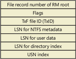
Figure 11-55 $TXF_DATA attribute.

The first field shown is the file record number of the root of the resource manager responsible for the transaction associated with this file. For the default resource manager, the file record number is 5, which is the file record number for the root directory (\) in the MFT, as shown earlier in Figure 11-31. TxF needs this information when it creates an FCB for the file so that it can link it to the correct resource manager, which in turn needs to create an enlistment for the transaction when a transacted file request is received by NTFS.

Another important piece of data stored in the $TXF_DATA attribute is the TxF file ID, or TxID, and this explains why $TXF_DATA attributes are never deleted. Because NTFS writes file names to its records when writing to the transaction log, it needs a way to uniquely identify files in the same directory that may have had the same name. For example, if sample.txt is deleted from a directory in a transaction and later a new file with the same name is created in the same directory (and as part of the same transaction), TxF needs a way to uniquely identify the two instances of sample.txt. This identification is provided by a 64-bit unique number, the TxID, that TxF increments when a new file (or an instance of a file) becomes part of a transaction. Because they can never be reused, TxIDs are permanent, so the $TXF_DATA attribute will never be removed from a file.

Last but not least, three CLFS (Common Logging File System) LSNs are stored for each file part of a transaction. Whenever a transaction is active, such as during create, rename, or write operations, TxF writes a log record to its CLFS log. Each record is assigned an LSN, and that LSN gets written to the appropriate field in the $TXF_DATA attribute. The first LSN is used to store the log record that identifies the changes to NTFS metadata in relation to this file. For example, if the standard attributes of a file are changed as part of a transacted operation, TxF must update the relevant MFT file record, and the LSN for the log record describing the change is stored. TxF uses the second LSN when the file’s data is modified. Finally, TxF uses the third LSN when the file name index for the directory requires a change related to a transaction the file took part in, or when a directory was part of a transaction and received a TxID.

The $TXF_DATA attribute also stores internal flags that describe the state information to TxF and the index of the USN record that was applied to the file on commit. A TxF transaction can span multiple USN records that may have been partly updated by NTFS’s recovery mechanism (described shortly), so the index tells TxF how many more USN records must be applied after a recovery.

TxF uses a default resource manager, one for each volume, to keep track of its transactional state. TxF, however, also supports additional resource managers called secondary resource managers. These resource managers can be defined by application writers and have their metadata located in any directory of the application’s choosing, defining their own transactional work units for undo, backup, restore, and redo operations. Both the default resource manager and secondary resource managers contain a number of metadata files and directories that describe their current state:

• ■    The $Txf directory, located into $Extend\$RmMetadata directory, which is where files are linked when they are deleted or overwritten by transactional operations.

• ■    The $Tops, or TxF Old Page Stream (TOPS) file, which contains a default data stream and an alternate data stream called $T. The default stream for the TOPS file contains metadata about the resource manager, such as its GUID, its CLFS log policy, and the LSN at which recovery should start. The $T stream contains file data that is partially overwritten by a transactional writer (as opposed to a full overwrite, which would move the file into the $Txf directory).

• ■    The TxF log files, which are CLFS log files storing transaction records. For the default resource manager, these files are part of the $TxfLog directory, but secondary resource managers can store them anywhere. TxF uses a multiplexed base log file called $TxfLog.blf. The file \$Extend\$RmMetadata\$TxfLog\$TxfLog contains two streams: the KtmLog stream used for Kernel Transaction Manager metadata records, and the TxfLog stream, which contains the TxF log records.

EXPERIMENT: Querying resource manager information

You can use the built-in Fsutil.exe command-line program to query information about the default resource manager as well as to create, start, and stop secondary resource managers and configure their logging policies and behaviors. The following command queries information about the default resource manager, which is identified by the root directory (\):

Click here to view code image

d:\>fsutil resource info \
    Resource Manager Identifier :      81E83020-E6FB-11E8-B862-D89EF33A38A7
    KTM Log Path for RM:  \Device\HarddiskVolume8\$Extend\$RmMetadata\$TxfLog\$TxfLog::KtmLog
    Space used by TOPS:   1 Mb
    TOPS free space:      100%
    RM State:             Active
    Running transactions: 0
    One phase commits:    0
    Two phase commits:    0
    System initiated rollbacks: 0
    Age of oldest transaction:  00:00:00
    Logging Mode:         Simple
    Number of containers: 2
    Container size:       10 Mb
    Total log capacity:   20 Mb
    Total free log space: 19 Mb
    Minimum containers:   2
    Maximum containers:   20
    Log growth increment: 2 container(s)
    Auto shrink:          Not enabled
    
    RM prefers availability over consistency.

As mentioned, the fsutil resource command has many options for configuring TxF resource managers, including the ability to create a secondary resource manager in any directory of your choice. For example, you can use the fsutil resource create c:\rmtest command to create a secondary resource manager in the Rmtest directory, followed by the fsutil resource start c:\rmtest command to initiate it. Note the presence of the $Tops and $TxfLogContainer* files and of the TxfLog and $Txf directories in this folder.

Logging implementation

As mentioned earlier, each time a change is made to the disk because of an ongoing transaction, TxF writes a record of the change to its log. TxF uses a variety of log record types to keep track of transactional changes, but regardless of the record type, all TxF log records have a generic header that contains information identifying the type of the record, the action related to the record, the TxID that the record applies to, and the GUID of the KTM transaction that the record is associated with.

A redo record specifies how to reapply a change part of a transaction that’s already been committed to the volume if the transaction has actually never been flushed from cache to disk. An undo record, on the other hand, specifies how to reverse a change part of a transaction that hasn’t been committed at the time of a rollback. Some records are redo-only, meaning they don’t contain any equivalent undo data, whereas other records contain both redo and undo information.

Through the TOPS file, TxF maintains two critical pieces of data, the base LSN and the restart LSN. The base LSN determines the LSN of the first valid record in the log, while the restart LSN indicates at which LSN recovery should begin when starting the resource manager. When TxF writes a restart record, it updates these two values, indicating that changes have been made to the volume and flushed out to disk—meaning that the file system is fully consistent up to the new restart LSN.

TxF also writes compensating log records, or CLRs. These records store the actions that are being performed during transaction rollback. They’re primarily used to store the undo-next LSN, which allows the recovery process to avoid repeated undo operations by bypassing undo records that have already been processed, a situation that can happen if the system fails during the recovery phase and has already performed part of the undo pass. Finally, TxF also deals with prepare records, abort records, and commit records, which describe the state of the KTM transactions related to TxF.

NTFS recovery support

NTFS recovery support ensures that if a power failure or a system failure occurs, no file system operations (transactions) will be left incomplete, and the structure of the disk volume will remain intact without the need to run a disk repair utility. The NTFS Chkdsk utility is used to repair catastrophic disk corruption caused by I/O errors (bad disk sectors, electrical anomalies, or disk failures, for example) or software bugs. But with the NTFS recovery capabilities in place, Chkdsk is rarely needed.

As mentioned earlier (in the section “Recoverability”), NTFS uses a transaction-processing scheme to implement recoverability. This strategy ensures a full disk recovery that is also extremely fast (on the order of seconds) for even the largest disks. NTFS limits its recovery procedures to file system data to ensure that at the very least the user will never lose a volume because of a corrupted file system; however, unless an application takes specific action (such as flushing cached files to disk), NTFS’s recovery support doesn’t guarantee user data to be fully updated if a crash occurs. This is the job of transactional NTFS (TxF).

The following sections detail the transaction-logging scheme NTFS uses to record modifications to file system data structures and explain how NTFS recovers a volume if the system fails.

Design

NTFS implements the design of a recoverable file system. These file systems ensure volume consistency by using logging techniques (sometimes called journaling) originally developed for transaction processing. If the operating system crashes, the recoverable file system restores consistency by executing a recovery procedure that accesses information that has been stored in a log file. Because the file system has logged its disk writes, the recovery procedure takes only seconds, regardless of the size of the volume (unlike in the FAT file system, where the repair time is related to the volume size). The recovery procedure for a recoverable file system is exact, guaranteeing that the volume will be restored to a consistent state.

A recoverable file system incurs some costs for the safety it provides. Every transaction that alters the volume structure requires that one record be written to the log file for each of the transaction’s suboperations. This logging overhead is ameliorated by the file system’s batching of log records—writing many records to the log file in a single I/O operation. In addition, the recoverable file system can employ the optimization techniques of a lazy write file system. It can even increase the length of the intervals between cache flushes because the file system metadata can be recovered if the system crashes before the cache changes have been flushed to disk. This gain over the caching performance of lazy write file systems makes up for, and often exceeds, the overhead of the recoverable file system’s logging activity.

Neither careful write nor lazy write file systems guarantee protection of user file data. If the system crashes while an application is writing a file, the file can be lost or corrupted. Worse, the crash can corrupt a lazy write file system, destroying existing files or even rendering an entire volume inaccessible.

The NTFS recoverable file system implements several strategies that improve its reliability over that of the traditional file systems. First, NTFS recoverability guarantees that the volume structure won’t be corrupted, so all files will remain accessible after a system failure. Second, although NTFS doesn’t guarantee protection of user data in the event of a system crash—some changes can be lost from the cache—applications can take advantage of the NTFS write-through and cache-flushing capabilities to ensure that file modifications are recorded on disk at appropriate intervals.

Both cache write-through—forcing write operations to be immediately recorded on disk—and cache flushing—forcing cache contents to be written to disk—are efficient operations. NTFS doesn’t have to do extra disk I/O to flush modifications to several different file system data structures because changes to the data structures are recorded—in a single write operation—in the log file; if a failure occurs and cache contents are lost, the file system modifications can be recovered from the log. Furthermore, unlike the FAT file system, NTFS guarantees that user data will be consistent and available immediately after a write-through operation or a cache flush, even if the system subsequently fails.

Metadata logging

NTFS provides file system recoverability by using the same logging technique used by TxF, which consists of recording all operations that modify file system metadata to a log file. Unlike TxF, however, NTFS’s built-in file system recovery support doesn’t make use of CLFS but uses an internal logging implementation called the log file service (which is not a background service process as described in Chapter 10). Another difference is that while TxF is used only when callers opt in for transacted operations, NTFS records all metadata changes so that the file system can be made consistent in the face of a system failure.

Log file service

The log file service (LFS) is a series of kernel-mode routines inside the NTFS driver that NTFS uses to access the log file. NTFS passes the LFS a pointer to an open file object, which specifies a log file to be accessed. The LFS either initializes a new log file or calls the Windows cache manager to access the existing log file through the cache, as shown in Figure 11-56. Note that although LFS and CLFS have similar sounding names, they’re separate logging implementations used for different purposes, although their operation is similar in many ways.

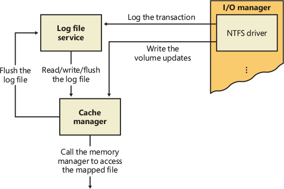
Figure 11-56 Log file service (LFS).

The LFS divides the log file into two regions: a restart area and an “infinite” logging area, as shown in Figure 11-57.

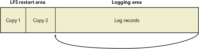
Figure 11-57 Log file regions.

NTFS calls the LFS to read and write the restart area. NTFS uses the restart area to store context information such as the location in the logging area at which NTFS begins to read during recovery after a system failure. The LFS maintains a second copy of the restart data in case the first becomes corrupted or otherwise inaccessible. The remainder of the log file is the logging area, which contains transaction records NTFS writes to recover a volume in the event of a system failure. The LFS makes the log file appear infinite by reusing it circularly (while guaranteeing that it doesn’t overwrite information it needs). Just like CLFS, the LFS uses LSNs to identify records written to the log file. As the LFS cycles through the file, it increases the values of the LSNs. NTFS uses 64 bits to represent LSNs, so the number of possible LSNs is so large as to be virtually infinite.

NTFS never reads transactions from or writes transactions to the log file directly. The LFS provides services that NTFS calls to open the log file, write log records, read log records in forward or backward order, flush log records up to a specified LSN, or set the beginning of the log file to a higher LSN. During recovery, NTFS calls the LFS to perform the same actions as described in the TxF recovery section: a redo pass for nonflushed committed changes, followed by an undo pass for noncommitted changes.

Here’s how the system guarantees that the volume can be recovered:

1. NTFS first calls the LFS to record in the (cached) log file any transactions that will modify the volume structure.

2. NTFS modifies the volume (also in the cache).

3. The cache manager prompts the LFS to flush the log file to disk. (The LFS implements the flush by calling the cache manager back, telling it which pages of memory to flush. Refer back to the calling sequence shown in Figure 11-56.)

4. After the cache manager flushes the log file to disk, it flushes the volume changes (the metadata operations themselves) to disk.

These steps ensure that if the file system modifications are ultimately unsuccessful, the corresponding transactions can be retrieved from the log file and can be either redone or undone as part of the file system recovery procedure.

File system recovery begins automatically the first time the volume is used after the system is rebooted. NTFS checks whether the transactions that were recorded in the log file before the crash were applied to the volume, and if they weren’t, it redoes them. NTFS also guarantees that transactions not completely logged before the crash are undone so that they don’t appear on the volume.

Log record types

The NTFS recovery mechanism uses similar log record types as the TxF recovery mechanism: update records, which correspond to the redo and undo records that TxF uses, and checkpoint records, which are similar to the restart records used by TxF. Figure 11-58 shows three update records in the log file. Each record represents one suboperation of a transaction, creating a new file. The redo entry in each update record tells NTFS how to reapply the suboperation to the volume, and the undo entry tells NTFS how to roll back (undo) the suboperation.

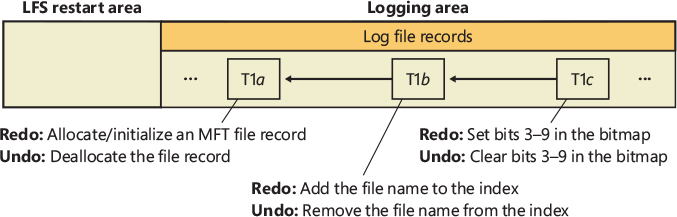
Figure 11-58 Update records in the log file.

After logging a transaction (in this example, by calling the LFS to write the three update records to the log file), NTFS performs the suboperations on the volume itself, in the cache. When it has finished updating the cache, NTFS writes another record to the log file, recording the entire transaction as complete—a suboperation known as committing a transaction. Once a transaction is committed, NTFS guarantees that the entire transaction will appear on the volume, even if the operating system subsequently fails.

When recovering after a system failure, NTFS reads through the log file and redoes each committed transaction. Although NTFS completed the committed transactions from before the system failure, it doesn’t know whether the cache manager flushed the volume modifications to disk in time. The updates might have been lost from the cache when the system failed. Therefore, NTFS executes the committed transactions again just to be sure that the disk is up to date.

After redoing the committed transactions during a file system recovery, NTFS locates all the transactions in the log file that weren’t committed at failure and rolls back each suboperation that had been logged. In Figure 11-58, NTFS would first undo the T1c suboperation and then follow the backward pointer to T1b and undo that suboperation. It would continue to follow the backward pointers, undoing suboperations, until it reached the first suboperation in the transaction. By following the pointers, NTFS knows how many and which update records it must undo to roll back a transaction.

Redo and undo information can be expressed either physically or logically. As the lowest layer of software maintaining the file system structure, NTFS writes update records with physical descriptions that specify volume updates in terms of particular byte ranges on the disk that are to be changed, moved, and so on, unlike TxF, which uses logical descriptions that express updates in terms of operations such as “delete file A.dat.” NTFS writes update records (usually several) for each of the following transactions:

• ■    Creating a file

• ■    Deleting a file

• ■    Extending a file

• ■    Truncating a file

• ■    Setting file information

• ■    Renaming a file

• ■    Changing the security applied to a file

The redo and undo information in an update record must be carefully designed because although NTFS undoes a transaction, recovers from a system failure, or even operates normally, it might try to redo a transaction that has already been done or, conversely, to undo a transaction that never occurred or that has already been undone. Similarly, NTFS might try to redo or undo a transaction consisting of several update records, only some of which are complete on disk. The format of the update records must ensure that executing redundant redo or undo operations is idempotent—that is, has a neutral effect. For example, setting a bit that is already set has no effect, but toggling a bit that has already been toggled does. The file system must also handle intermediate volume states correctly.

In addition to update records, NTFS periodically writes a checkpoint record to the log file, as illustrated in Figure 11-59.

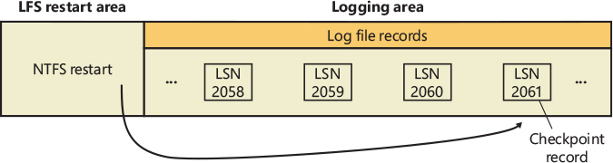
Figure 11-59 Checkpoint record in the log file.

A checkpoint record helps NTFS determine what processing would be needed to recover a volume if a crash were to occur immediately. Using information stored in the checkpoint record, NTFS knows, for example, how far back in the log file it must go to begin its recovery. After writing a checkpoint record, NTFS stores the LSN of the record in the restart area so that it can quickly find its most recently written checkpoint record when it begins file system recovery after a crash occurs; this is similar to the restart LSN used by TxF for the same reason.

Although the LFS presents the log file to NTFS as if it were infinitely large, it isn’t. The generous size of the log file and the frequent writing of checkpoint records (an operation that usually frees up space in the log file) make the possibility of the log file filling up a remote one. Nevertheless, the LFS, just like CLFS, accounts for this possibility by tracking several operational parameters:

• ■    The available log space

• ■    The amount of space needed to write an incoming log record and to undo the write, should that be necessary

• ■    The amount of space needed to roll back all active (noncommitted) transactions, should that be necessary

If the log file doesn’t contain enough available space to accommodate the total of the last two items, the LFS returns a “log file full” error, and NTFS raises an exception. The NTFS exception handler rolls back the current transaction and places it in a queue to be restarted later.

To free up space in the log file, NTFS must momentarily prevent further transactions on files. To do so, NTFS blocks file creation and deletion and then requests exclusive access to all system files and shared access to all user files. Gradually, active transactions either are completed successfully or receive the “log file full” exception. NTFS rolls back and queues the transactions that receive the exception.

Once it has blocked transaction activity on files as just described, NTFS calls the cache manager to flush unwritten data to disk, including unwritten log file data. After everything is safely flushed to disk, NTFS no longer needs the data in the log file. It resets the beginning of the log file to the current position, making the log file “empty.” Then it restarts the queued transactions. Beyond the short pause in I/O processing, the log file full error has no effect on executing programs.

This scenario is one example of how NTFS uses the log file not only for file system recovery but also for error recovery during normal operation. You find out more about error recovery in the following section.

Recovery

NTFS automatically performs a disk recovery the first time a program accesses an NTFS volume after the system has been booted. (If no recovery is needed, the process is trivial.) Recovery depends on two tables NTFS maintains in memory: a transaction table, which behaves just like the one TxF maintains, and a dirty page table, which records which pages in the cache contain modifications to the file system structure that haven’t yet been written to disk. This data must be flushed to disk during recovery.

NTFS writes a checkpoint record to the log file once every 5 seconds. Just before it does, it calls the LFS to store a current copy of the transaction table and of the dirty page table in the log file. NTFS then records in the checkpoint record the LSNs of the log records containing the copied tables. When recovery begins after a system failure, NTFS calls the LFS to locate the log records containing the most recent checkpoint record and the most recent copies of the transaction and dirty page tables. It then copies the tables to memory.

The log file usually contains more update records following the last checkpoint record. These update records represent volume modifications that occurred after the last checkpoint record was written. NTFS must update the transaction and dirty page tables to include these operations. After updating the tables, NTFS uses the tables and the contents of the log file to update the volume itself.

To perform its volume recovery, NTFS scans the log file three times, loading the file into memory during the first pass to minimize disk I/O. Each pass has a particular purpose:

1. Analysis

2. Redoing transactions

3. Undoing transactions

Analysis pass

During the analysis pass, as shown in Figure 11-60, NTFS scans forward in the log file from the beginning of the last checkpoint operation to find update records and use them to update the transaction and dirty page tables it copied to memory. Notice in the figure that the checkpoint operation stores three records in the log file and that update records might be interspersed among these records. NTFS therefore must start its scan at the beginning of the checkpoint operation.

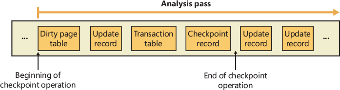
Figure 11-60 Analysis pass.

Most update records that appear in the log file after the checkpoint operation begins represent a modification to either the transaction table or the dirty page table. If an update record is a “transaction committed” record, for example, the transaction the record represents must be removed from the transaction table. Similarly, if the update record is a page update record that modifies a file system data structure, the dirty page table must be updated to reflect that change.

Once the tables are up to date in memory, NTFS scans the tables to determine the LSN of the oldest update record that logs an operation that hasn’t been carried out on disk. The transaction table contains the LSNs of the noncommitted (incomplete) transactions, and the dirty page table contains the LSNs of records in the cache that haven’t been flushed to disk. The LSN of the oldest update record that NTFS finds in these two tables determines where the redo pass will begin. If the last checkpoint record is older, however, NTFS will start the redo pass there instead.

Note

In the TxF recovery model, there is no distinct analysis pass. Instead, as described in the TxF recovery section, TxF performs the equivalent work in the redo pass.

Redo pass

During the redo pass, as shown in Figure 11-61, NTFS scans forward in the log file from the LSN of the oldest update record, which it found during the analysis pass. It looks for page update records, which contain volume modifications that were written before the system failure but that might not have been flushed to disk. NTFS redoes these updates in the cache.

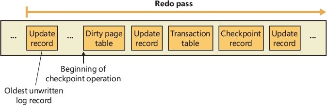
Figure 11-61 Redo pass.

When NTFS reaches the end of the log file, it has updated the cache with the necessary volume modifications, and the cache manager’s lazy writer can begin writing cache contents to disk in the background.

Undo pass

After it completes the redo pass, NTFS begins its undo pass, in which it rolls back any transactions that weren’t committed when the system failed. Figure 11-62 shows two transactions in the log file; transaction 1 was committed before the power failure, but transaction 2 wasn’t. NTFS must undo transaction 2.

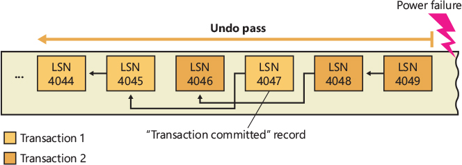
Figure 11-62 Undo pass.

Suppose that transaction 2 created a file, an operation that comprises three suboperations, each with its own update record. The update records of a transaction are linked by backward pointers in the log file because they aren’t usually contiguous.

The NTFS transaction table lists the LSN of the last-logged update record for each noncommitted transaction. In this example, the transaction table identifies LSN 4049 as the last update record logged for transaction 2. As shown from right to left in Figure 11-63, NTFS rolls back transaction 2.

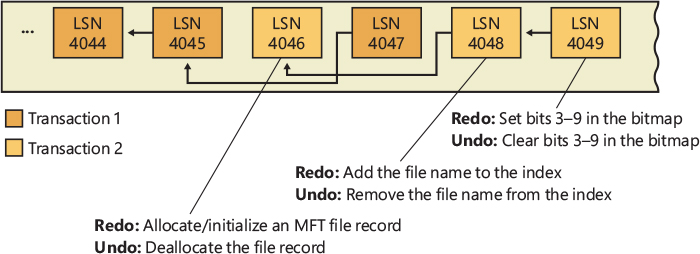
Figure 11-63 Undoing a transaction.

After locating LSN 4049, NTFS finds the undo information and executes it, clearing bits 3 through 9 in its allocation bitmap. NTFS then follows the backward pointer to LSN 4048, which directs it to remove the new file name from the appropriate file name index. Finally, it follows the last backward pointer and deallocates the MFT file record reserved for the file, as the update record with LSN 4046 specifies. Transaction 2 is now rolled back. If there are other noncommitted transactions to undo, NTFS follows the same procedure to roll them back. Because undoing transactions affects the volume’s file system structure, NTFS must log the undo operations in the log file. After all, the power might fail again during the recovery, and NTFS would have to redo its undo operations!

When the undo pass of the recovery is finished, the volume has been restored to a consistent state. At this point, NTFS is prepared to flush the cache changes to disk to ensure that the volume is up to date. Before doing so, however, it executes a callback that TxF registers for notifications of LFS flushes. Because TxF and NTFS both use write-ahead logging, TxF must flush its log through CLFS before the NTFS log is flushed to ensure consistency of its own metadata. (And similarly, the TOPS file must be flushed before the CLFS-managed log files.) NTFS then writes an “empty” LFS restart area to indicate that the volume is consistent and that no recovery need be done if the system should fail again immediately. Recovery is complete.

NTFS guarantees that recovery will return the volume to some preexisting consistent state, but not necessarily to the state that existed just before the system crash. NTFS can’t make that guarantee because, for performance, it uses a lazy commit algorithm, which means that the log file isn’t immediately flushed to disk each time a transaction committed record is written. Instead, numerous transaction committed records are batched and written together, either when the cache manager calls the LFS to flush the log file to disk or when the LFS writes a checkpoint record (once every 5 seconds) to the log file. Another reason the recovered volume might not be completely up to date is that several parallel transactions might be active when the system crashes, and some of their transaction committed records might make it to disk, whereas others might not. The consistent volume that recovery produces includes all the volume updates whose transaction committed records made it to disk and none of the updates whose transaction committed records didn’t make it to disk.

NTFS uses the log file to recover a volume after the system fails, but it also takes advantage of an important freebie it gets from logging transactions. File systems necessarily contain a lot of code devoted to recovering from file system errors that occur during the course of normal file I/O. Because NTFS logs each transaction that modifies the volume structure, it can use the log file to recover when a file system error occurs and thus can greatly simplify its error handling code. The log file full error described earlier is one example of using the log file for error recovery.

Most I/O errors that a program receives aren’t file system errors and therefore can’t be resolved entirely by NTFS. When called to create a file, for example, NTFS might begin by creating a file record in the MFT and then enter the new file’s name in a directory index. When it tries to allocate space for the file in its bitmap, however, it could discover that the disk is full and the create request can’t be completed. In such a case, NTFS uses the information in the log file to undo the part of the operation it has already completed and to deallocate the data structures it reserved for the file. Then it returns a disk full error to the caller, which in turn must respond appropriately to the error.

NTFS bad-cluster recovery

The volume manager included with Windows (VolMgr) can recover data from a bad sector on a fault-tolerant volume, but if the hard disk doesn’t perform bad-sector remapping or runs out of spare sectors, the volume manager can’t perform bad-sector replacement to replace the bad sector. When the file system reads from the sector, the volume manager instead recovers the data and returns the warning to the file system that there is only one copy of the data.

The FAT file system doesn’t respond to this volume manager warning. Moreover, neither FAT nor the volume manager keeps track of the bad sectors, so a user must run the Chkdsk or Format utility to prevent the volume manager from repeatedly recovering data for the file system. Both Chkdsk and Format are less than ideal for removing bad sectors from use. Chkdsk can take a long time to find and remove bad sectors, and Format wipes all the data off the partition it’s formatting.

In the file system equivalent of a volume manager’s bad-sector replacement, NTFS dynamically replaces the cluster containing a bad sector and keeps track of the bad cluster so that it won’t be reused. (Recall that NTFS maintains portability by addressing logical clusters rather than physical sectors.) NTFS performs these functions when the volume manager can’t perform bad-sector replacement. When a volume manager returns a bad-sector warning or when the hard disk driver returns a bad-sector error, NTFS allocates a new cluster to replace the one containing the bad sector. NTFS copies the data that the volume manager has recovered into the new cluster to reestablish data redundancy.

Figure 11-64 shows an MFT record for a user file with a bad cluster in one of its data runs as it existed before the cluster went bad. When it receives a bad-sector error, NTFS reassigns the cluster containing the sector to its bad-cluster file, $BadClus. This prevents the bad cluster from being allocated to another file. NTFS then allocates a new cluster for the file and changes the file’s VCN-to-LCN mappings to point to the new cluster. This bad-cluster remapping (introduced earlier in this chapter) is illustrated in Figure 11-64. Cluster number 1357, which contains the bad sector, must be replaced by a good cluster.

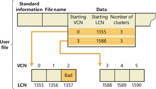
Figure 11-64 MFT record for a user file with a bad cluster.

Bad-sector errors are undesirable, but when they do occur, the combination of NTFS and the volume manager provides the best possible solution. If the bad sector is on a redundant volume, the volume manager recovers the data and replaces the sector if it can. If it can’t replace the sector, it returns a warning to NTFS, and NTFS replaces the cluster containing the bad sector.

If the volume isn’t configured as a redundant volume, the data in the bad sector can’t be recovered. When the volume is formatted as a FAT volume and the volume manager can’t recover the data, reading from the bad sector yields indeterminate results. If some of the file system’s control structures reside in the bad sector, an entire file or group of files (or potentially, the whole disk) can be lost. At best, some data in the affected file (often, all the data in the file beyond the bad sector) is lost. Moreover, the FAT file system is likely to reallocate the bad sector to the same or another file on the volume, causing the problem to resurface.

Like the other file systems, NTFS can’t recover data from a bad sector without help from a volume manager. However, NTFS greatly contains the damage a bad sector can cause. If NTFS discovers the bad sector during a read operation, it remaps the cluster the sector is in, as shown in Figure 11-65. If the volume isn’t configured as a redundant volume, NTFS returns a data read error to the calling program. Although the data that was in that cluster is lost, the rest of the file—and the file system—remains intact; the calling program can respond appropriately to the data loss, and the bad cluster won’t be reused in future allocations. If NTFS discovers the bad cluster on a write operation rather than a read, NTFS remaps the cluster before writing and thus loses no data and generates no error.

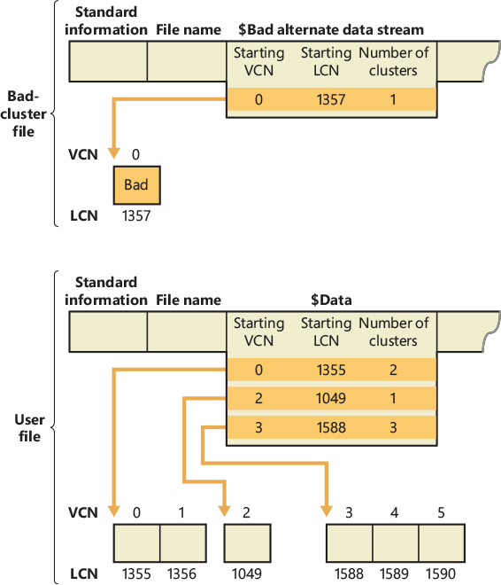
Figure 11-65 Bad-cluster remapping.

The same recovery procedures are followed if file system data is stored in a sector that goes bad. If the bad sector is on a redundant volume, NTFS replaces the cluster dynamically, using the data recovered by the volume manager. If the volume isn’t redundant, the data can’t be recovered, so NTFS sets a bit in the $Volume metadata file that indicates corruption on the volume. The NTFS Chkdsk utility checks this bit when the system is next rebooted, and if the bit is set, Chkdsk executes, repairing the file system corruption by reconstructing the NTFS metadata.

In rare instances, file system corruption can occur even on a fault-tolerant disk configuration. A double error can destroy both file system data and the means to reconstruct it. If the system crashes while NTFS is writing the mirror copy of an MFT file record—of a file name index or of the log file, for example—the mirror copy of such file system data might not be fully updated. If the system were rebooted and a bad-sector error occurred on the primary disk at exactly the same location as the incomplete write on the disk mirror, NTFS would be unable to recover the correct data from the disk mirror. NTFS implements a special scheme for detecting such corruptions in file system data. If it ever finds an inconsistency, it sets the corruption bit in the volume file, which causes Chkdsk to reconstruct the NTFS metadata when the system is next rebooted. Because file system corruption is rare on a fault-tolerant disk configuration, Chkdsk is seldom needed. It is supplied as a safety precaution rather than as a first-line data recovery strategy.

The use of Chkdsk on NTFS is vastly different from its use on the FAT file system. Before writing anything to disk, FAT sets the volume’s dirty bit and then resets the bit after the modification is complete. If any I/O operation is in progress when the system crashes, the dirty bit is left set and Chkdsk runs when the system is rebooted. On NTFS, Chkdsk runs only when unexpected or unreadable file system data is found, and NTFS can’t recover the data from a redundant volume or from redundant file system structures on a single volume. (The system boot sector is duplicated—in the last sector of a volume—as are the parts of the MFT ($MftMirr) required for booting the system and running the NTFS recovery procedure. This redundancy ensures that NTFS will always be able to boot and recover itself.)

Table 11-11 summarizes what happens when a sector goes bad on a disk volume formatted for one of the Windows-supported file systems according to various conditions we’ve described in this section.

Table 11-11 Summary of NTFS data recovery scenarios

Scenario	With a Disk That Supports Bad-Sector Remapping and Has Spare Sectors	With a Disk That Does Not Perform Bad-Sector Remapping or Has No Spare Sectors
Fault-tolerant volume1	Volume manager recovers the data. Volume manager performs bad-sector replacement. File system remains unaware of the error.	Volume manager recovers the data. Volume manager sends the data and a bad-sector error to the file system. NTFS performs cluster remapping.
Non-fault-tolerant volume	Volume manager can’t recover the data. Volume manager sends a bad-sector error to the file system. NTFS performs cluster remapping. Data is lost.2	Volume manager can’t recover the data. Volume manager sends a bad-sector error to the file system. NTFS performs cluster remapping. Data is lost.

1 A fault-tolerant volume is one of the following: a mirror set (RAID-1) or a RAID-5 set.

2 In a write operation, no data is lost: NTFS remaps the cluster before the write.

If the volume on which the bad sector appears is a fault-tolerant volume—a mirrored (RAID-1) or RAID-5 / RAID-6 volume—and if the hard disk is one that supports bad-sector replacement (and that hasn’t run out of spare sectors), it doesn’t matter which file system you’re using (FAT or NTFS). The volume manager replaces the bad sector without the need for user or file system intervention.

If a bad sector is located on a hard disk that doesn’t support bad sector replacement, the file system is responsible for replacing (remapping) the bad sector or—in the case of NTFS—the cluster in which the bad sector resides. The FAT file system doesn’t provide sector or cluster remapping. The benefits of NTFS cluster remapping are that bad spots in a file can be fixed without harm to the file (or harm to the file system, as the case may be) and that the bad cluster will never be used again.

Self-healing

With today’s multiterabyte storage devices, taking a volume offline for a consistency check can result in a service outage of many hours. Recognizing that many disk corruptions are localized to a single file or portion of metadata, NTFS implements a self-healing feature to repair damage while a volume remains online. When NTFS detects corruption, it prevents access to the damaged file or files and creates a system worker thread that performs Chkdsk-like corrections to the corrupted data structures, allowing access to the repaired files when it has finished. Access to other files continues normally during this operation, minimizing service disruption.

You can use the fsutil repair set command to view and set a volume’s repair options, which are summarized in Table 11-12. The Fsutil utility uses the FSCTL_SET_REPAIR file system control code to set these settings, which are saved in the VCB for the volume.

Table 11-12 NTFS self-healing behaviors

Flag	Behavior
SET_REPAIR_ENABLED	Enable self-healing for the volume.
SET_REPAIR_WARN_ABOUT_DATA_LOSS	If the self-healing process is unable to fully recover a file, specifies whether the user should be visually warned.
SET_REPAIR_DISABLED_AND_BUGCHECK_ON_CORRUPTION	If the NtfsBugCheckOnCorrupt NTFS registry value was set by using fsutil behavior set NtfsBugCheckOnCorrupt 1 and this flag is set, the system will crash with a STOP error 0x24, indicating file system corruption. This setting is automatically cleared during boot time to avoid repeated reboot cycles.

In all cases, including when the visual warning is disabled (the default), NTFS will log any self-healing operation it undertook in the System event log.

Apart from periodic automatic self-healing, NTFS also supports manually initiated self-healing cycles (this type of self-healing is called proactive) through the FSCTL_INITIATE_REPAIR and FSCTL_WAIT_FOR_REPAIR control codes, which can be initiated with the fsutil repair initiate and fsutil repair wait commands. This allows the user to force the repair of a specific file and to wait until repair of that file is complete.

To check the status of the self-healing mechanism, the FSCTL_QUERY_REPAIR control code or the fsutil repair query command can be used, as shown here:

Click here to view code image

C:\>fsutil repair query c:
    Self healing state on c: is: 0x9
    
     Values: 0x1 - Enable general repair.
             0x9 - Enable repair and warn about potential data loss.
            0x10 - Disable repair and bugcheck once on first corruption.

Online check-disk and fast repair

Rare cases in which disk-corruptions are not managed by the NTFS file system driver (through self-healing, Log file service, and so on) require the system to run the Windows Check Disk tool and to put the volume offline. There are a variety of unique causes for disk corruption: whether they are caused by media errors from the hard disk or transient memory errors, corruptions can happen in file system metadata. In large file servers, which have multiple terabytes of disk space, running a complete Check Disk can require days. Having a volume offline for so long in these kinds of scenarios is typically not acceptable.

Before Windows 8, NTFS implemented a simpler health model, where the file system volume was either healthy or not (through the dirty bit stored in the $VOLUME_INFORMATION attribute). In that model, the volume was taken offline for as long as necessary to fix the file system corruptions and bring the volume back to a healthy state. Downtime was directly proportional to the number of files in the volume. Windows 8, with the goal of reducing or avoiding the downtime caused by file system corruption, has redesigned the NTFS health model and disk check.

The new model introduces new components that cooperate to provide an online check-disk tool and to drastically reduce the downtime in case severe file-system corruption is detected. The NTFS file system driver is able to identify multiple types of corruption during normal system I/O. If a corruption is detected, NTFS tries to self-heal it (see the previous paragraph). If it doesn’t succeed, the NTFS file system driver writes a new corruption record to the $Verify stream of the \$Extend\$RmMetadata\$Repair file.

A corruption record is a common data structure that NTFS uses for describing metadata corruptions and is used both in-memory and on-disk. A corruption record is represented by a fixed-size header, which contains version information, flags, and uniquely represents the record type through a GUID, a variable-sized description for the type of corruption that occurred, and an optional context.

After the entry has been correctly added, NTFS emits an ETW event through its own event provider (named Microsoft-Windows-Ntfs-UBPM). This ETW event is consumed by the service control manager, which will start the Spot Verifier service (more details about triggered-start services are available in Chapter 10).

The Spot Verifier service (implemented in the Svsvc.dll library) verifies that the signaled corruption is not a false positive (some corruptions are intermittent due to memory issues and may not be a result of an actual corruption on disk). Entries in the $Verify stream are removed while being verified by the Spot Verifier. If the corruption (described by the entry) is not a false positive, the Spot Verifier triggers the Proactive Scan Bit (P-bit) in the $VOLUME_INFORMATION attribute of the volume, which will trigger an online scan of the file system. The online scan is executed by the Proactive Scanner, which is run as a maintenance task by the Windows task scheduler (the task is located in Microsoft\Windows\Chkdsk, as shown in Figure 11-66) when the time is appropriate.

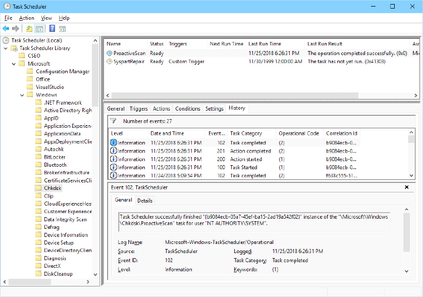
Figure 11-66 The Proactive Scan maintenance task.

The Proactive scanner is implemented in the Untfs.dll library, which is imported by the Windows Check Disk tool (Chkdsk.exe). When the Proactive Scanner runs, it takes a snapshot of the target volume through the Volume Shadow Copy service and runs a complete Check Disk on the shadow volume. The shadow volume is read-only; the check disk code detects this and, instead of directly fixing the errors, uses the self-healing feature of NTFS to try to automatically fix the corruption. If it fails, it sends a FSCTL_CORRUPTION_HANDLING code to the file system driver, which in turn creates an entry in the $Corrupt stream of the \$Extend\$RmMetadata\$Repair metadata file and sets the volume’s dirty bit.

The dirty bit has a slightly different meaning compared to previous editions of Windows. The $VOLUME_INFORMATION attribute of the NTFS root namespace still contains the dirty bit, but also contains the P-bit, which is used to require a Proactive Scan, and the F-bit, which is used to require a full check disk due to the severity of a particular corruption. The dirty bit is set to 1 by the file system driver if the P-bit or the F-bit are enabled, or if the $Corrupt stream contains one or more corruption records.

If the corruption is still not resolved, at this stage there are no other possibilities to fix it when the volume is offline (this does not necessarily require an immediate volume unmounting). The Spot Fixer is a new component that is shared between the Check Disk and the Autocheck tool. The Spot Fixer consumes the records inserted in the $Corrupt stream by the Proactive scanner. At boot time, the Autocheck native application detects that the volume is dirty, but, instead of running a full check disk, it fixes only the corrupted entries located in the $Corrupt stream, an operation that requires only a few seconds. Figure 11-67 shows a summary of the different repair methodology implemented in the previously described components of the NTFS file system.

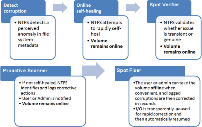
Figure 11-67 A scheme that describes the components that cooperate to provide online check disk and fast corruption repair for NTFS volumes.

A Proactive scan can be manually started for a volume through the chkdsk /scan command. In the same way, the Spot Fixer can be executed by the Check Disk tool using the /spotfix command-line argument.

EXPERIMENT: Testing the online disk check

You can test the online checkdisk by performing a simple experiment. Assuming that you would like to execute an online checkdisk on the D: volume, start by playing a large video stream from the D drive. In the meantime, open an administrative command prompt window and start an online checkdisk through the following command:

Click here to view code image

C:\>chkdsk d: /scan
    The type of the file system is NTFS.
    Volume label is DATA.
    
    Stage 1: Examining basic file system structure ...
      4041984 file records processed.
    File verification completed.
      3778 large file records processed.
      0 bad file records processed.
    
    Stage 2: Examining file name linkage ...
    Progress: 3454102 of 4056090 done; Stage: 85%; Total: 51%; ETA:   0:00:43 ..

You will find that the video stream won’t be stopped and continues to play smoothly. In case the online checkdisk finds an error that it isn’t able to correct while the volume is mounted, it will be inserted in the $Corrupt stream of the $Repair system file. To fix the errors, a volume dismount is needed, but the correction will be very fast. In that case, you could simply reboot the machine or manually execute the Spot Fixer through the command line:

C:\>chkdsk d: /spotfix

In case you choose to execute the Spot Fixer, you will find that the video stream will be interrupted, because the volume needs to be unmounted.

Encrypted file system

Windows includes a full-volume encryption feature called Windows BitLocker Drive Encryption. BitLocker encrypts and protects volumes from offline attacks, but once a system is booted, BitLocker’s job is done. The Encrypting File System (EFS) protects individual files and directories from other authenticated users on a system. When choosing how to protect your data, it is not an either/or choice between BitLocker and EFS; each provides protection from specific—and nonoverlapping—threats. Together, BitLocker and EFS provide a “defense in depth” for the data on your system.

The paradigm used by EFS is to encrypt files and directories using symmetric encryption (a single key that is used for encrypting and decrypting the file). The symmetric encryption key is then encrypted using asymmetric encryption (one key for encryption—often referred to as the public key—and a different key for decryption—often referred to as the private key) for each user who is granted access to the file. The details and theory behind these encryption methods is beyond the scope of this book; however, a good primer is available at https://docs.microsoft.com/en-us/windows/desktop/SecCrypto/cryptography-essentials.

EFS works with the Windows Cryptography Next Generation (CNG) APIs, and thus may be configured to use any algorithm supported by (or added to) CNG. By default, EFS will use the Advanced Encryption Standard (AES) for symmetric encryption (256-bit key) and the Rivest-Shamir-Adleman (RSA) public key algorithm for asymmetric encryption (2,048-bit keys).

Users can encrypt files via Windows Explorer by opening a file’s Properties dialog box, clicking Advanced, and then selecting the Encrypt Contents To Secure Data option, as shown in Figure 11-68. (A file may be encrypted or compressed, but not both.) Users can also encrypt files via a command-line utility named Cipher (%SystemRoot%\System32\Cipher.exe) or programmatically using Windows APIs such as EncryptFile and AddUsersToEncryptedFile.

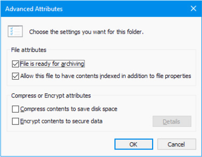
Figure 11-68 Encrypt files by using the Advanced Attributes dialog box.

Windows automatically encrypts files that reside in directories that are designated as encrypted directories. When a file is encrypted, EFS generates a random number for the file that EFS calls the file’s File Encryption Key (FEK). EFS uses the FEK to encrypt the file’s contents using symmetric encryption. EFS then encrypts the FEK using the user’s asymmetric public key and stores the encrypted FEK in the $EFS alternate data stream for the file. The source of the public key may be administratively specified to come from an assigned X.509 certificate or a smartcard or can be randomly generated (which would then be added to the user’s certificate store, which can be viewed using the Certificate Manager (%SystemRoot%\System32\Certmgr.msc). After EFS completes these steps, the file is secure; other users can’t decrypt the data without the file’s decrypted FEK, and they can’t decrypt the FEK without the user private key.

Symmetric encryption algorithms are typically very fast, which makes them suitable for encrypting large amounts of data, such as file data. However, symmetric encryption algorithms have a weakness: You can bypass their security if you obtain the key. If multiple users want to share one encrypted file protected only using symmetric encryption, each user would require access to the file’s FEK. Leaving the FEK unencrypted would obviously be a security problem, but encrypting the FEK once would require all the users to share the same FEK decryption key—another potential security problem.

Keeping the FEK secure is a difficult problem, which EFS addresses with the public key–based half of its encryption architecture. Encrypting a file’s FEK for individual users who access the file lets multiple users share an encrypted file. EFS can encrypt a file’s FEK with each user’s public key and can store each user’s encrypted FEK in the file’s $EFS data stream. Anyone can access a user’s public key, but no one can use a public key to decrypt the data that the public key encrypted. The only way users can decrypt a file is with their private key, which the operating system must access. A user’s private key decrypts the user’s encrypted copy of a file’s FEK. Public key–based algorithms are usually slow, but EFS uses these algorithms only to encrypt FEKs. Splitting key management between a publicly available key and a private key makes key management a little easier than symmetric encryption algorithms do and solves the dilemma of keeping the FEK secure.

Several components work together to make EFS work, as the diagram of EFS architecture in Figure 11-69 shows. EFS support is merged into the NTFS driver. Whenever NTFS encounters an encrypted file, NTFS executes EFS functions that it contains. The EFS functions encrypt and decrypt file data as applications access encrypted files. Although EFS stores an FEK with a file’s data, users’ public keys encrypt the FEK. To encrypt or decrypt file data, EFS must decrypt the file’s FEK with the aid of CNG key management services that reside in user mode.

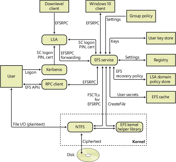
Figure 11-69 EFS architecture.

The Local Security Authority Subsystem (LSASS, %SystemRoot%\System32\Lsass.exe) manages logon sessions but also hosts the EFS service (Efssvc.dll). For example, when EFS needs to decrypt a FEK to decrypt file data a user wants to access, NTFS sends a request to the EFS service inside LSASS.

Encrypting a file for the first time

The NTFS driver calls its EFS helper functions when it encounters an encrypted file. A file’s attributes record that the file is encrypted in the same way that a file records that it’s compressed (discussed earlier in this chapter). NTFS has specific interfaces for converting a file from nonencrypted to encrypted form, but user-mode components primarily drive the process. As described earlier, Windows lets you encrypt a file in two ways: by using the cipher command-line utility or by checking the Encrypt Contents To Secure Data check box in the Advanced Attributes dialog box for a file in Windows Explorer. Both Windows Explorer and the cipher command rely on the EncryptFile Windows API.

EFS stores only one block of information in an encrypted file, and that block contains an entry for each user sharing the file. These entries are called key entries, and EFS stores them in the data decryption field (DDF) portion of the file’s EFS data. A collection of multiple key entries is called a key ring because, as mentioned earlier, EFS lets multiple users share encrypted files.

Figure 11-70 shows a file’s EFS information format and key entry format. EFS stores enough information in the first part of a key entry to precisely describe a user’s public key. This data includes the user’s security ID (SID) (note that the SID is not guaranteed to be present), the container name in which the key is stored, the cryptographic provider name, and the asymmetric key pair certificate hash. Only the asymmetric key pair certificate hash is used by the decryption process. The second part of the key entry contains an encrypted version of the FEK. EFS uses the CNG to encrypt the FEK with the selected asymmetric encryption algorithm and the user’s public key.

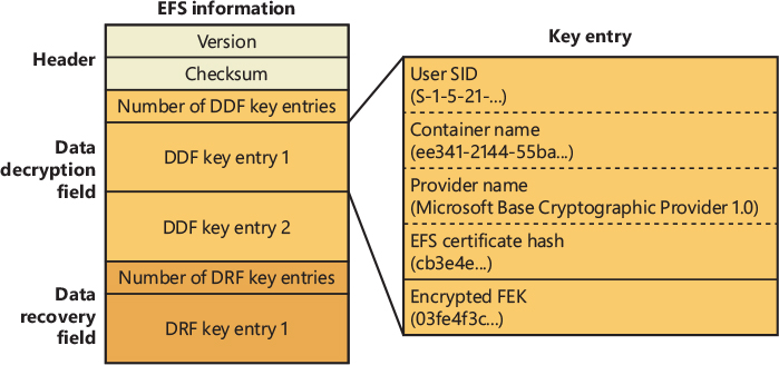
Figure 11-70 Format of EFS information and key entries.

EFS stores information about recovery key entries in a file’s data recovery field (DRF). The format of DRF entries is identical to the format of DDF entries. The DRF’s purpose is to let designated accounts, or recovery agents, decrypt a user’s file when administrative authority must have access to the user’s data. For example, suppose a company employee forgot his or her logon password. An administrator can reset the user’s password, but without recovery agents, no one can recover the user’s encrypted data.

Recovery agents are defined with the Encrypted Data Recovery Agents security policy of the local computer or domain. This policy is available from the Local Security Policy MMC snap-in, as shown in Figure 11-71. When you use the Add Recovery Agent Wizard (by right-clicking Encrypting File System and then clicking Add Data Recovery Agent), you can add recovery agents and specify which private/public key pairs (designated by their certificates) the recovery agents use for EFS recovery. Lsasrv (Local Security Authority service, which is covered in Chapter 7 of Part 1) interprets the recovery policy when it initializes and when it receives notification that the recovery policy has changed. EFS creates a DRF key entry for each recovery agent by using the cryptographic provider registered for EFS recovery.

Figure 11-71 Encrypted Data Recovery Agents group policy.

A user can create their own Data Recovery Agent (DRA) certificate by using the cipher /r command. The generated private certificate file can be imported by the Recovery Agent Wizard and by the Certificates snap-in of the domain controller or the machine on which the administrator should be able to decrypt encrypted files.

As the final step in creating EFS information for a file, Lsasrv calculates a checksum for the DDF and DRF by using the MD5 hash facility of Base Cryptographic Provider 1.0. Lsasrv stores the checksum’s result in the EFS information header. EFS references this checksum during decryption to ensure that the contents of a file’s EFS information haven’t become corrupted or been tampered with.

Encrypting file data

When a user encrypts an existing file, the following process occurs:

1. The EFS service opens the file for exclusive access.

2. All data streams in the file are copied to a plaintext temporary file in the system’s temporary directory.

3. A FEK is randomly generated and used to encrypt the file by using AES-256.

4. A DDF is created to contain the FEK encrypted by using the user’s public key. EFS automatically obtains the user’s public key from the user’s X.509 version 3 file encryption certificate.

5. If a recovery agent has been designated through Group Policy, a DRF is created to contain the FEK encrypted by using RSA and the recovery agent’s public key.

6. EFS automatically obtains the recovery agent’s public key for file recovery from the recovery agent’s X.509 version 3 certificate, which is stored in the EFS recovery policy. If there are multiple recovery agents, a copy of the FEK is encrypted by using each agent’s public key, and a DRF is created to store each encrypted FEK.

   Note

   The file recovery property in the certificate is an example of an enhanced key usage (EKU) field. An EKU extension and extended property specify and limit the valid uses of a certificate. File Recovery is one of the EKU fields defined by Microsoft as part of the Microsoft public key infrastructure (PKI).

7. EFS writes the encrypted data, along with the DDF and the DRF, back to the file. Because symmetric encryption does not add additional data, file size increase is minimal after encryption. The metadata, consisting primarily of encrypted FEKs, is usually less than 1 KB. File size in bytes before and after encryption is normally reported to be the same.

8. The plaintext temporary file is deleted.

When a user saves a file to a folder that has been configured for encryption, the process is similar except that no temporary file is created.

The decryption process

When an application accesses an encrypted file, decryption proceeds as follows:

1. NTFS recognizes that the file is encrypted and sends a request to the EFS driver.

2. The EFS driver retrieves the DDF and passes it to the EFS service.

3. The EFS service retrieves the user’s private key from the user’s profile and uses it to decrypt the DDF and obtain the FEK.

4. The EFS service passes the FEK back to the EFS driver.

5. The EFS driver uses the FEK to decrypt sections of the file as needed for the application.

   Note

   When an application opens a file, only those sections of the file that the application is using are decrypted because EFS uses cipher block chaining. The behavior is different if the user removes the encryption attribute from the file. In this case, the entire file is decrypted and rewritten as plaintext.

6. The EFS driver returns the decrypted data to NTFS, which then sends the data to the requesting application.

Backing up encrypted files

An important aspect of any file encryption facility’s design is that file data is never available in unencrypted form except to applications that access the file via the encryption facility. This restriction particularly affects backup utilities, in which archival media store files. EFS addresses this problem by providing a facility for backup utilities so that the utilities can back up and restore files in their encrypted states. Thus, backup utilities don’t have to be able to decrypt file data, nor do they need to encrypt file data in their backup procedures.

Backup utilities use the EFS API functions OpenEncryptedFileRaw, ReadEncryptedFileRaw, WriteEncryptedFileRaw, and CloseEncryptedFileRaw in Windows to access a file’s encrypted contents. After a backup utility opens a file for raw access during a backup operation, the utility calls ReadEncryptedFileRaw to obtain the file data. All the EFS backup utilities APIs work by issuing FSCTL to the NTFS file system. For example, the ReadEncryptedFileRaw API first reads the $EFS stream by issuing a FSCTL_ENCRYPTION_FSCTL_IO control code to the NTFS driver and then reads all of the file’s streams (including the $DATA stream and optional alternate data streams); in case the stream is encrypted, the ReadEncryptedFileRaw API uses the FSCTL_READ_RAW_ENCRYPTED control code to request the encrypted stream data to the file system driver.

EXPERIMENT: Viewing EFS information

EFS has a handful of other API functions that applications can use to manipulate encrypted files. For example, applications use the AddUsersToEncryptedFile API function to give additional users access to an encrypted file and RemoveUsersFromEncryptedFile to revoke users’ access to an encrypted file. Applications use the QueryUsersOnEncryptedFile function to obtain information about a file’s associated DDF and DRF key fields. QueryUsersOnEncryptedFile returns the SID, certificate hash value, and display information that each DDF and DRF key field contains. The following output is from the EFSDump utility, from Sysinternals, when an encrypted file is specified as a command-line argument:

Click here to view code image

C:\Andrea>efsdump Test.txt
    EFS Information Dumper v1.02
    Copyright (C) 1999 Mark Russinovich
    Systems Internals - http://www.sysinternals.com
    
    C:\Andrea\Test.txt:
    DDF Entries:
        WIN-46E4EFTBP6Q\Andrea:
            Andrea(Andrea@WIN-46E4EFTBP6Q)
        Unknown user:
            Tony(Tony@WIN-46E4EFTBP6Q)
    DRF Entry:
        Unknown user:
            EFS Data Recovery

You can see that the file Test.txt has two DDF entries for the users Andrea and Tony and one DRF entry for the EFS Data Recovery agent, which is the only recovery agent currently registered on the system. You can use the cipher tool to add or remove users in the DDF entries of a file. For example, the command

Click here to view code image

cipher /adduser /user:Tony Test.txt

enables the user Tony to access the encrypted file Test.txt (adding an entry in the DDF of the file).

Copying encrypted files

When an encrypted file is copied, the system doesn’t decrypt the file and re-encrypt it at its destination; it just copies the encrypted data and the EFS alternate data stream to the specified destination. However, if the destination does not support alternate data streams—if it is not an NTFS volume (such as a FAT volume) or is a network share (even if the network share is an NTFS volume)—the copy cannot proceed normally because the alternate data streams would be lost. If the copy is done with Explorer, a dialog box informs the user that the destination volume does not support encryption and asks the user whether the file should be copied to the destination unencrypted. If the user agrees, the file will be decrypted and copied to the specified destination. If the copy is done from a command prompt, the copy command will fail and return the error message “The specified file could not be encrypted.”

BitLocker encryption offload

The NTFS file system driver uses services provided by the Encrypting File System (EFS) to perform file encryption and decryption. These kernel-mode services, which communicate with the user-mode encrypting file service (Efssvc.dll), are provided to NTFS through callbacks. When a user or application encrypts a file for the first time, the EFS service sends a FSCTL_SET_ENCRYPTION control code to the NTFS driver. The NTFS file system driver uses the “write” EFS callback to perform in-memory encryption of the data located in the original file. The actual encryption process is performed by splitting the file content, which is usually processed in 2-MB blocks, in small 512-byte chunks. The EFS library uses the BCryptEncrypt API to actually encrypt the chunk. As previously mentioned, the encryption engine is provided by the Kernel CNG driver (Cng.sys), which supports the AES or 3DES algorithms used by EFS (along with many more). As EFS encrypts each 512-byte chunk (which is the smallest physical size of standard hard disk sectors), at every round it updates the IV (initialization vector, also known as salt value, which is a 128-bit number used to provide randomization to the encryption scheme), using the byte offset of the current block.

In Windows 10, encryption performance has increased thanks to BitLocker encryption offload. When BitLocker is enabled, the storage stack already includes a device created by the Full Volume Encryption Driver (Fvevol.sys), which, if the volume is encrypted, performs real-time encryption/decryption on physical disk sectors; otherwise, it simply passes through the I/O requests.

The NTFS driver can defer the encryption of a file by using IRP Extensions. IRP Extensions are provided by the I/O manager (more details about the I/O manager are available in Chapter 6 of Part 1) and are a way to store different types of additional information in an IRP. At file creation time, the EFS driver probes the device stack to check whether the BitLocker control device object (CDO) is present (by using the IOCTL_FVE_GET_CDOPATH control code), and, if so, it sets a flag in the SCB, indicating that the stream can support encryption offload.

Every time an encrypted file is read or written, or when a file is encrypted for the first time, the NTFS driver, based on the previously set flag, determines whether it needs to encrypt/decrypt each file block. In case encryption offload is enabled, NTFS skips the call to EFS; instead, it adds an IRP extension to the IRP that will be sent to the related volume device for performing the physical I/O. In the IRP extension, the NTFS file system driver stores the starting virtual byte offset of the block of the file that the storage driver is going to read or write, its size, and some flags. The NTFS driver finally emits the I/O to the related volume device by using the IoCallDriver API.

The volume manager will parse the IRP and send it to the correct storage driver. The BitLocker driver recognizes the IRP extension and encrypts the data that NTFS has sent down to the device stack, using its own routines, which operate on physical sectors. (Bitlocker, as a volume filter driver, doesn’t implement the concept of files and directories.) Some storage drivers, such as the Logical Disk Manager driver (VolmgrX.sys, which provides dynamic disk support) are filter drivers that attach to the volume device objects. These drivers reside below the volume manager but above the BitLocker driver, and they can provide data redundancy, striping, or storage virtualization, characteristics which are usually implemented by splitting the original IRP into multiple secondary IRPs that will be emitted to different physical disk devices. In this case, the secondary I/Os, when intercepted by the BitLocker driver, will result in data encrypted by using a different salt value that would corrupt the file data.

IRP extensions support the concept of IRP propagation, which automatically modifies the file virtual byte offset stored in the IRP extension every time the original IRP is split. Normally, the EFS driver encrypts file blocks on 512-byte boundaries, and the IRP can’t be split on an alignment less than a sector size. As a result, BitLocker can correctly encrypt and decrypt the data, ensuring that no corruption will happen.

Many of BitLocker driver’s routines can’t tolerate memory failures. However, since IRP extension is dynamically allocated from the nonpaged pool when the IRP is split, the allocation can fail. The I/O manager resolves this problem with the IoAllocateIrpEx routine. This routine can be used by kernel drivers for allocating IRPs (like the legacy IoAllocateIrp). But the new routine allocates an extra stack location and stores any IRP extensions in it. Drivers that request an IRP extension on IRPs allocated by the new API no longer need to allocate new memory from the nonpaged pool.

Note

A storage driver can decide to split an IRP for different reasons—whether or not it needs to send multiple I/Os to multiple physical devices. The Volume Shadow Copy Driver (Volsnap.sys), for example, splits the I/O while it needs to read a file from a copy-on-write volume shadow copy, if the file resides in different sections: on the live volume and on the Shadow Copy’s differential file (which resides in the System Volume Information hidden directory).

Online encryption support

When a file stream is encrypted or decrypted, it is exclusively locked by the NTFS file system driver. This means that no applications can access the file during the entire encryption or decryption process. For large files, this limitation can break the file’s availability for many seconds—or even minutes. Clearly this is not acceptable for large file-server environments.

To resolve this, recent versions of Windows 10 introduced online encryption support. Through the right synchronization, the NTFS driver is able to perform file encryption and decryption without retaining exclusive file access. EFS enables online encryption only if the target encryption stream is a data stream (named or unnamed) and is nonresident. (Otherwise, a standard encryption process starts.) If both conditions are satisfied, the EFS service sends a FSCTL_SET_ENCRYPTION control code to the NTFS driver to set a flag that enables online encryption.

Online encryption is possible thanks to the "$EfsBackup" attribute (of type $LOGGED_UTILITY_STREAM) and to the introduction of range locks, a new feature that allows the file system driver to lock (in an exclusive or shared mode) only only a portion of a file. When online encryption is enabled, the NtfsEncryptDecryptOnline internal function starts the encryption and decryption process by creating the $EfsBackup attribute (and its SCB) and by acquiring a shared lock on the first 2-MB range of the file. A shared lock means that multiple readers can still read from the file range, but other writers need to wait until the end of the encryption or decryption operation before they can write new data.

The NTFS driver allocates a 2-MB buffer from the nonpaged pool and reserves some clusters from the volume, which are needed to represent 2 MB of free space. (The total number of clusters depends on the volume cluster’s size.) The online encryption function reads the original data from the physical disk and stores it in the allocated buffer. If BitLocker encryption offload is not enabled (described in the previous section), the buffer is encrypted using EFS services; otherwise, the BitLocker driver encrypts the data when the buffer is written to the previously reserved clusters.

At this stage, NTFS locks the entire file for a brief amount of time: only the time needed to remove the clusters containing the unencrypted data from the original stream’s extent table, assign them to the $EfsBackup non-resident attribute, and replace the removed range of the original stream’s extent table with the new clusters that contain the newly encrypted data. Before releasing the exclusive lock, the NTFS driver calculates a new high watermark value and stores it both in the original file in-memory SCB and in the EFS payload of the $EFS alternate data stream. NTFS then releases the exclusive lock. The clusters that contain the original data are first zeroed out; then, if there are no more blocks to process, they are eventually freed. Otherwise, the online encryption cycle restarts with the next 2-MB chunk.

The high watermark value stores the file offset that represents the boundary between encrypted and nonencrypted data. Any concurrent write beyond the watermark can occur in its original form; other concurrent writes before the watermark need to be encrypted before they can succeed. Writes to the current locked range are not allowed. Figure 11-72 shows an example of an ongoing online encryption for a 16-MB file. The first two blocks (2 MB in size) already have been encrypted; the high watermark value is set to 4 MB, dividing the file between its encrypted and non-encrypted data. A range lock is set on the 2-MB block that follows the high watermark. Applications can still read from that block, but they can’t write any new data (in the latter case, they need to wait). The block’s data is encrypted and stored in reserved clusters. When exclusive file ownership is taken, the original block’s clusters are remapped to the $EfsBackup stream (by removing or splitting their entry in the original file’s extent table and inserting a new entry in the $EfsBackup attribute), and the new clusters are inserted in place of the previous ones. The high watermark value is increased, the file lock is released, and the online encryption process proceeds to the next stage starting at the 6-MB offset; the previous clusters located in the $EfsBackup stream are concurrently zeroed-out and can be reused for new stages.

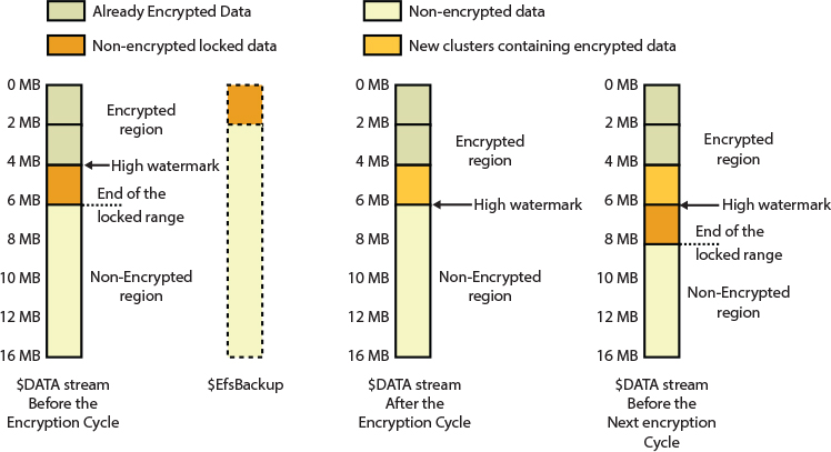
Figure 11-72 Example of an ongoing online encryption for a 16MB file.

The new implementation allows NTFS to encrypt or decrypt in place, getting rid of temporary files (see the previous “Encrypting file data” section for more details). More importantly, it allows NTFS to perform file encryption and decryption while other applications can still use and modify the target file stream (the time spent with the exclusive lock hold is small and not perceptible by the application that is attempting to use the file).

Direct Access (DAX) disks

Persistent memory is an evolution of solid-state disk technology: a new kind of nonvolatile storage medium that has RAM-like performance characteristics (low latency and high bandwidth), resides on the memory bus (DDR), and can be used like a standard disk device.

Direct Access Disks (DAX) is the term used by the Windows operating system to refer to such persistent memory technology (another common term used is storage class memory, abbreviated as SCM). A nonvolatile dual in-line memory module (NVDIMM), shown in Figure 11-73, is an example of this new type of storage. NVDIMM is a type of memory that retains its contents even when electrical power is removed. “Dual in-line” identifies the memory as using DIMM packaging. At the time of writing, there are three different types of NVDIMMs: NVIDIMM-F contains only flash storage; NVDIMM-N, the most common, is produced by combining flash storage and traditional DRAM chips on the same module; and NVDIMM-P has persistent DRAM chips, which do not lose data in event of power failure.

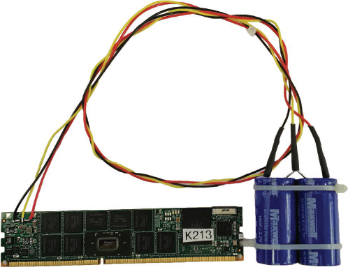
Figure 11-73 An NVDIMM, which has DRAM and Flash chips. An attached battery or on-board supercapacitors are needed for maintaining the data in the DRAM chips.

One of the main characteristics of DAX, which is key to its fast performance, is the support of zero-copy access to persistent memory. This means that many components, like the file system driver and memory manager, need to be updated to support DAX, which is a disruptive technology.

Windows Server 2016 was the first Windows operating system to supports DAX: the new storage model provides compatibility with most existing applications, which can run on DAX disks without any modification. For fastest performance, files and directories on a DAX volume need to be mapped in memory using memory-mapped APIs, and the volume needs to be formatted in a special DAX mode. At the time of this writing, only NTFS supports DAX volumes.

The following sections describe the way in which direct access disks operate and detail the architecture of the new driver model and the modification on the main components responsible for DAX volume support: the NTFS driver, memory manager, cache manager, and I/O manager. Additionally, inbox and third-party file system filter drivers (including mini filters) must also be individually updated to take full advantage of DAX.

DAX driver model

To support DAX volumes, Windows needed to introduce a brand-new storage driver model. The SCM Bus Driver (Scmbus.sys) is a new bus driver that enumerates physical and logical persistent memory (PM) devices on the system, which are attached to its memory bus (the enumeration is performed thanks to the NFIT ACPI table). The bus driver, which is not considered part of the I/O path, is a primary bus driver managed by the ACPI enumerator, which is provided by the HAL (hardware abstraction layer) through the hardware database registry key (HKLM\SYSTEM\CurrentControlSet\Enum\ACPI). More details about Plug & Play Device enumeration are available in Chapter 6 of Part 1.

Figure 11-74 shows the architecture of the SCM storage driver model. The SCM bus driver creates two different types of device objects:

• ■    Physical device objects (PDOs) represent physical PM devices. A NVDIMM device is usually composed of one or multiple interleaved NVDIMM-N modules. In the former case, the SCM bus driver creates only one physical device object representing the NVDIMM unit. In the latter case, it creates two distinct devices that represent each NVDIMM-N module. All the physical devices are managed by the miniport driver, Nvdimm.sys, which controls a physical NVDIMM and is responsible for monitoring its health.

• ■    Functional device objects (FDOs) represent single DAX disks, which are managed by the persistent memory driver, Pmem.sys. The driver controls any byte-addressable interleave sets and is responsible for all I/O directed to a DAX volume. The persistent memory driver is the class driver for each DAX disk. (It replaces Disk.sys in the classical storage stack.)

Both the SCM bus driver and the NVDIMM miniport driver expose some interfaces for communication with the PM class driver. Those interfaces are exposed through an IRP_MJ_PNP major function by using the IRP_MN_QUERY_INTERFACE request. When the request is received, the SCM bus driver knows that it should expose its communication interface because callers specify the {8de064ff-b630-42e4-ea88-6f24c8641175} interface GUID. Similarly, the persistent memory driver requires communication interface to the NVDIMM devices through the {0079c21b-917e-405e-cea9-0732b5bbcebd} GUID.

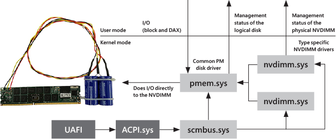
Figure 11-74 The SCM Storage driver model.

The new storage driver model implements a clear separation of responsibilities: The PM class driver manages logical disk functionality (open, close, read, write, memory mapping, and so on), whereas NVDIMM drivers manage the physical device and its health. It will be easy in the future to add support for new types of NVDIMM by just updating the Nvdimm.sys driver. (Pmem.sys doesn’t need to change.)

DAX volumes

The DAX storage driver model introduces a new kind of volume: the DAX volumes. When a user first formats a partition through the Format tool, she can specify the /DAX argument to the command line. If the underlying medium is a DAX disk, and it’s partitioned using the GPT scheme, before creating the basic disk data structure needed for the NTFS file system, the tool writes the GPT_BASIC_DATA_ ATTRIBUTE_DAX flag in the target volume GPT partition entry (which corresponds to bit number 58). A good reference for the GUID partition table is available at https://en.wikipedia.org/wiki/GUID_Partition_Table.

When the NTFS driver then mounts the volume, it recognizes the flag and sends a STORAGE_QUERY_PROPERTY control code to the underlying storage driver. The IOCTL is recognized by the SCM bus driver, which responds to the file system driver with another flag specifying that the underlying disk is a DAX disk. Only the SCM bus driver can set the flag. Once the two conditions are verified, and as long as DAX support is not disabled through the HKLM\System\CurrentControlSet\Control\FileSystem\NtfsEnableDirectAccess registry value, NTFS enables DAX volume support.

DAX volumes are different from the standard volumes mainly because they support zero-copy access to the persistent memory. Memory-mapped files provide applications with direct access to the underlying hardware disk sectors (through a mapped view), meaning that no intermediary components will intercept any I/O. This characteristic provides extreme performance (but as mentioned earlier, can impact file system filter drivers, including minifilters).

When an application creates a memory-mapped section backed by a file that resides on a DAX volume, the memory manager asks the file system whether the section should be created in DAX mode, which is true only if the volume has been formatted in DAX mode, too. When the file is later mapped through the MapViewOfFile API, the memory manager asks the file system for the physical memory range of a given range of the file. The file system driver translates the requested file range in one or more volume relative extents (sector offset and length) and asks the PM disk class driver to translate the volume extents into physical memory ranges. The memory manager, after receiving the physical memory ranges, updates the target process page tables for the section to map directly to persistent storage. This is a truly zero-copy access to storage: an application has direct access to the persistent memory. No paging reads or paging writes will be generated. This is important; the cache manager is not involved in this case. We examine the implications of this later in the chapter.

Applications can recognize DAX volumes by using the GetVolumeInformation API. If the returned flags include FILE_DAX_VOLUME, the volume is formatted with a DAX-compatible file system (only NTFS at the time of this writing). In the same way, an application can identify whether a file resides on a DAX disk by using the GetVolumeInformationByHandle API.

Cached and noncached I/O in DAX volumes

Even though memory-mapped I/O for DAX volumes provide zero-copy access to the underlying storage, DAX volumes still support I/O through standard means (via classic ReadFile and WriteFile APIs). As described at the beginning of the chapter, Windows supports two kinds of regular I/O: cached and noncached. Both types have significant differences when issued to DAX volumes.

Cached I/O still requires interaction from the cache manager, which, while creating a shared cache map for the file, requires the memory manager to create a section object that directly maps to the PM hardware. NTFS is able to communicate to the cache manager that the target file is in DAX-mode through the new CcInitializeCacheMapEx routine. The cache manager will then copy data from the user buffer to persistent memory: cached I/O has therefore one-copy access to persistent storage. Note that cached I/O is still coherent with other memory-mapped I/O (the cache manager uses the same section); as in the memory-mapped I/O case, there are still no paging reads or paging writes, so the lazy writer thread and intelligent read-ahead are not enabled.

One implication of the direct-mapping is that the cache manager directly writes to the DAX disk as soon as the NtWriteFile function completes. This means that cached I/O is essentially noncached. For this reason, noncached I/O requests are directly converted by the file system to cached I/O such that the cache manager still copies directly between the user’s buffer and persistent memory. This kind of I/O is still coherent with cached and memory-mapped I/O.

NTFS continues to use standard I/O while processing updates to its metadata files. DAX mode I/O for each file is decided at stream creation time by setting a flag in the stream control block. If a file is a system metadata file, the attribute is never set, so the cache manager, when mapping such a file, creates a standard non-DAX file-backed section, which will use the standard storage stack for performing paging read or write I/Os. (Ultimately, each I/O is processed by the Pmem driver just like for block volumes, using the sector atomicity algorithm. See the “Block volumes” section for more details.) This behavior is needed for maintaining compatibility with write-ahead logging. Metadata must not be persisted to disk before the corresponding log is flushed. So, if a metadata file were DAX mapped, that write-ahead logging requirement would be broken.

Effects on file system functionality

The absence of regular paging I/O and the application’s ability to directly access persistent memory eliminate traditional hook points that the file systems and related filters use to implement various features. Multiple functionality cannot be supported on DAX-enabled volumes, like file encryption, compressed and sparse files, snapshots, and USN journal support.

In DAX mode, the file system no longer knows when a writable memory-mapped file is modified. When the memory section is first created, the NTFS file system driver updates the file’s modification and access times and marks the file as modified in the USN change journal. At the same time, it signals a directory change notification. DAX volumes are no longer compatible with any kind of legacy filter drivers and have a big impact on minifilters (filter manager clients). Components like BitLocker and the volume shadow copy driver (Volsnap.sys) don’t work with DAX volumes and are removed from the device stack. Because a minifilter no longer knows if a file has been modified, an antimalware file access scanner, such as one described earlier, can no longer know if it should scan a file for viruses. It needs to assume, on any handle close, that modification may have occurred. In turn, this significantly harms performance, so minifilters must manually opt-in to support DAX volumes.

Mapping of executable images

When the Windows loader maps an executable image into memory, it uses memory-mapping services provided by the memory manager. The loader creates a memory-mapped image section by supplying the SEC_IMAGE flag to the NtCreateSection API. The flag specifies to the loader to map the section as an image, applying all the necessary fixups. In DAX mode this mustn’t be allowed to happen; otherwise, all the relocations and fixups will be applied to the original image file on the PM disk. To correctly deal with this problem, the memory manager applies the following strategies while mapping an executable image stored in a DAX mode volume:

• ■    If there is already a control area that represents a data section for the binary file (meaning that an application has opened the image for reading binary data), the memory manager creates an empty memory-backed image section and copies the data from the existing data section to the newly created image section; then it applies the necessary fixups.

• ■    If there are no data sections for the file, the memory manager creates a regular non-DAX image section, which creates standard invalid prototype PTEs (see Chapter 5 of Part 1 for more details). In this case, the memory manager uses the standard read and write routines of the Pmem driver to bring data in memory when a page fault for an invalid access on an address that belongs to the image-backed section happens.

At the time of this writing, Windows 10 does not support execution in-place, meaning that the loader is not able to directly execute an image from DAX storage. This is not a problem, though, because DAX mode volumes have been originally designed to store data in a very performant way. Execution in-place for DAX volumes will be supported in future releases of Windows.

EXPERIMENT: Witnessing DAX I/O with Process Monitor

You can witness DAX I/Os using Process Monitor from SysInternals and the FsTool.exe application, which is available in this book’s downloadable resources. When an application reads or writes from a memory-mapped file that resides on a DAX-mode volume, the system does not generate any paging I/O, so nothing is visible to the NTFS driver or to the minifilters that are attached above or below it. To witness the described behavior, just open Process Monitor, and, assuming that you have two different volumes mounted as the P: and Q: drives, set the filters in a similar way as illustrated in the following figure (the Q: drive is the DAX-mode volume):

For generating I/O on DAX-mode volumes, you need to simulate a DAX copy using the FsTool application. The following example copies an ISO image located in the P: DAX block-mode volume (even a standard volume created on the top of a regular disk is fine for the experiment) to the DAX-mode “Q:” drive:

Click here to view code image

P:\>fstool.exe /daxcopy p:\Big_image.iso q:\test.iso
    NTFS / ReFS Tool v0.1
    Copyright (C) 2018 Andrea Allievi (AaLl86)
    
    Starting DAX copy...
       Source file path: p:\Big_image.iso.
       Target file path: q:\test.iso.
       Source Volume: p:\ - File system: NTFS - Is DAX Volume: False.
       Target Volume: q:\ - File system: NTFS - Is DAX Volume: True.
    
       Source file size: 4.34 GB
    
    Performing file copy... Success!
       Total execution time: 8 Sec.
       Copy Speed: 489.67 MB/Sec
    
    Press any key to exit...

Process Monitor has captured a trace of the DAX copy operation that confirms the expected results:

From the trace above, you can see that on the target file (Q:\test.iso), only the CreateFileMapping operation was intercepted: no WriteFile events are visible. While the copy was proceeding, only paging I/O on the source file was detected by Process Monitor. These paging I/Os were generated by the memory manager, which needed to read the data back from the source volume as the application was generating page faults while accessing the memory-mapped file.

To see the differences between memory-mapped I/O and standard cached I/O, you need to copy again the file using a standard file copy operation. To see paging I/O on the source file data, make sure to restart your system; otherwise, the original data remains in the cache:

Click here to view code image

P:\>fstool.exe /copy p:\Big_image.iso q:\test.iso
    NTFS / ReFS Tool v0.1
    Copyright (C) 2018 Andrea Allievi (AaLl86)
    
    Copying "Big_image.iso" to "test.iso" file... Success.
       Total File-Copy execution time: 13 Sec - Transfer Rate: 313.71 MB/s.
    Press any key to exit...

If you compare the trace acquired by Process Monitor with the previous one, you can confirm that cached I/O is a one-copy operation. The cache manager still copies chunks of memory between the application-provided buffer and the system cache, which is mapped directly on the DAX disk. This is confirmed by the fact that again, no paging I/O is highlighted on the target file.

As a last experiment, you can try to start a DAX copy between two files that reside on the same DAX-mode volume or that reside on two different DAX-mode volumes:

Click here to view code image

P:\>fstool /daxcopy q:\test.iso q:\test_copy_2.iso
    TFS / ReFS Tool v0.1
    Copyright (C) 2018 Andrea Allievi (AaLl86)
    
    Starting DAX copy...
       Source file path: q:\test.iso.
       Target file path: q:\test_copy_2.iso.
       Source Volume: q:\ - File system: NTFS - Is DAX Volume: True.
       Target Volume: q:\ - File system: NTFS - Is DAX Volume: True.
    Great! Both the source and the destination reside on a DAX volume.
    Performing a full System Speed Copy!
    
       Source file size: 4.34 GB
    
    Performing file copy... Success!
       Total execution time: 8 Sec.
       Copy Speed: 501.60 MB/Sec
    
    Press any key to exit...

The trace collected in the last experiment demonstrates that memory-mapped I/O on DAX volumes doesn’t generate any paging I/O. No WriteFile or ReadFile events are visible on either the source or the target file:

Block volumes

Not all the limitations brought on by DAX volumes are acceptable in certain scenarios. Windows provides backward compatibility for PM hardware through block-mode volumes, which are managed by the entire legacy I/O stack as regular volumes used by rotating and SSD disk. Block volumes maintain existing storage semantics: all I/O operations traverse the storage stack on the way to the PM disk class driver. (There are no miniport drivers, though, because they’re not needed.) They’re fully compatible with all existing applications, legacy filters, and minifilter drivers.

Persistent memory storage is able to perform I/O at byte granularity. More accurately, I/O is performed at cache line granularity, which depends on the architecture but is usually 64 bytes. However, block mode volumes are exposed as standard volumes, which perform I/O at sector granularity (512 bytes or 4 Kbytes). If a write is in progress on a DAX volume, and suddenly the drive experiences a power failure, the block of data (sector) contains a mix of old and new data. Applications are not prepared to handle such a scenario. In block mode, the sector atomicity is guaranteed by the PM disk class driver, which implements the Block Translation Table (BTT) algorithm.

The BTT, an algorithm developed by Intel, splits available disk space into chunks of up to 512 GB, called arenas. For each arena, the algorithm maintains a BTT, a simple indirection/lookup that maps an LBA to an internal block belonging to the arena. For each 32-bit entry in the map, the algorithm uses the two most significant bits (MSB) to store the status of the block (three states: valid, zeroed, and error). Although the table maintains the status of each LBA, the BTT algorithm provides sector atomicity by providing a flog area, which contains an array of nfree blocks.

An nfree block contains all the data that the algorithm needs to provide sector atomicity. There are 256 nfree entries in the array; an nfree entry is 32 bytes in size, so the flog area occupies 8 KB. Each nfree is used by one CPU, so the number of nfrees describes the number of concurrent atomic I/Os an arena can process concurrently. Figure 11-75 shows the layout of a DAX disk formatted in block mode. The data structures used for the BTT algorithm are not visible to the file system driver. The BTT algorithm eliminates possible subsector torn writes and, as described previously, is needed even on DAX-formatted volumes in order to support file system metadata writes.

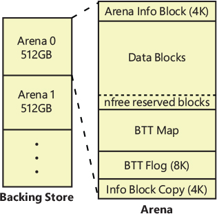
Figure 11-75 Layout of a DAX disk that supports sector atomicity (BTT algorithm).

Block mode volumes do not have the GPT_BASIC_DATA_ATTRIBUTE_DAX flag in their partition entry. NTFS behaves just like with normal volumes by relying on the cache manager to perform cached I/O, and by processing non-cached I/O through the PM disk class driver. The Pmem driver exposes read and write functions, which performs a direct memory access (DMA) transfer by building a memory descriptor list (MDL) for both the user buffer and device physical block address (MDLs are described in more detail in Chapter 5 of Part 1). The BTT algorithm provides sector atomicity. Figure 11-76 shows the I/O stack of a traditional volume, a DAX volume, and a block volume.

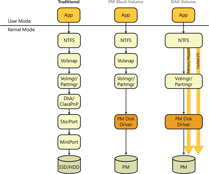
Figure 11-76 Device I/O stack comparison between traditional volumes, block mode volumes, and DAX volumes.

File system filter drivers and DAX

Legacy filter drivers and minifilters don’t work with DAX volumes. These kinds of drivers usually augment file system functionality, often interacting with all the operations that a file system driver manages. There are different classes of filters providing new capabilities or modifying existing functionality of the file system driver: antivirus, encryption, replication, compression, Hierarchical Storage Management (HSM), and so on. The DAX driver model significantly modifies how DAX volumes interact with such components.

As previously discussed in this chapter, when a file is mapped in memory, the file system in DAX mode does not receive any read or write I/O requests, neither do all the filter drivers that reside above or below the file system driver. This means that filter drivers that rely on data interception will not work. To minimize possible compatibility issues, existing minifilters will not receive a notification (through the InstanceSetup callback) when a DAX volume is mounted. New and updated minifilter drivers that still want to operate with DAX volumes need to specify the FLTFL_REGISTRATION_SUPPORT_DAX_VOLUME flag when they register with the filter manager through FltRegisterFilter kernel API.

Minifilters that decide to support DAX volumes have the limitation that they can’t intercept any form of paging I/O. Data transformation filters (which provide encryption or compression) don’t have any chance of working correctly for memory-mapped files; antimalware filters are impacted as described earlier—because they must now perform scans on every open and close, losing the ability to determine whether or not a write truly happened. (The impact is mostly tied to the detection of a file last update time.) Legacy filters are no longer compatible: if a driver calls the IoAttachDeviceToDevice Stack API (or similar functions), the I/O manager simply fails the request (and logs an ETW event).

Flushing DAX mode I/Os

Traditional disks (HDD, SSD, NVme) always include a cache that improves their overall performance. When write I/Os are emitted from the storage driver, the actual data is first transferred into the cache, which will be written to the persistent medium later. The operating system provides correct flushing, which guarantees that data is written to final storage, and temporal order, which guarantees that data is written in the correct order. For normal cached I/O, an application can call the FlushFileBuffers API to ensure that the data is provably stored on the disk (this will generate an IRP with the IRP_MJ_FLUSH_BUFFERS major function code that the NTFS driver will implement). Noncached I/O is directly written to disk by NTFS so ordering and flushing aren’t concerns.

With DAX-mode volumes, this is not possible anymore. After the file is mapped in memory, the NTFS driver has no knowledge of the data that is going to be written to disk. If an application is writing some critical data structures on a DAX volume and the power fails, the application has no guarantees that all of the data structures will have been correctly written in the underlying medium. Furthermore, it has no guarantees that the order in which the data was written was the requested one. This is because PM storage is implemented as classical physical memory from the CPU’s point of view. The processor uses the CPU caching mechanism, which uses its own caching mechanisms while reading or writing to DAX volumes.

As a result, newer versions of Windows 10 had to introduce new flush APIs for DAX-mapped regions, which perform the necessary work to optimally flush PM content from the CPU cache. The APIs are available for both user-mode applications and kernel-mode drivers and are highly optimized based on the CPU architecture (standard x64 systems use the CLFLUSH and CLWB opcodes, for example). An application that wants I/O ordering and flushing on DAX volumes can call RtlGetNonVolatileToken on a PM mapped region; the function yields back a nonvolatile token that can be subsequently used with the RtlFlushNonVolatileMemory or RtlFlushNonVolatileMemoryRanges APIs. Both APIs perform the actual flush of the data from the CPU cache to the underlying PM device.

Memory copy operations executed using standard OS functions perform, by default, temporal copy operations, meaning that data always passes through the CPU cache, maintaining execution ordering. Nontemporal copy operations, on the other hand, use specialized processor opcodes (again depending on the CPU architecture; x64 CPUs use the MOVNTI opcode) to bypass the CPU cache. In this case, ordering is not maintained, but execution is faster. RtlWriteNonVolatileMemory exposes memory copy operations to and from nonvolatile memory. By default, the API performs classical temporal copy operations, but an application can request a nontemporal copy through the WRITE_NV_MEMORY_FLAG_NON_ TEMPORAL flag and thus execute a faster copy operation.

Large and huge pages support

Reading or writing a file on a DAX-mode volume through memory-mapped sections is handled by the memory manager in a similar way to non-DAX sections: if the MEM_LARGE_PAGES flag is specified at map time, the memory manager detects that one or more file extents point to enough aligned, contiguous physical space (NTFS allocates the file extents), and uses large (2 MB) or huge (1 GB) pages to map the physical DAX space. (More details on the memory manager and large pages are available in Chapter 5 of Part 1.) Large and huge pages have various advantages compared to traditional 4-KB pages. In particular, they boost the performance on DAX files because they require fewer lookups in the processor’s page table structures and require fewer entries in the processor’s translation lookaside buffer (TLB). For applications with a large memory footprint that randomly access memory, the CPU can spend a lot of time looking up TLB entries as well as reading and writing the page table hierarchy in case of TLB misses. In addition, using large/huge pages can also result in significant commit savings because only page directory parents and page directory (for large files only, not huge files) need to be charged. Page table space (4 KB per 2 MB of leaf VA space) charges are not needed or taken. So, for example, with a 2-TB file mapping, the system can save 4 GB of committed memory by using large and huge pages.

The NTFS driver cooperates with the memory manager to provide support for huge and large pages while mapping files that reside on DAX volumes:

• ■    By default, each DAX partition is aligned on 2-MB boundaries.

• ■    NTFS supports 2-MB clusters. A DAX volume formatted with 2-MB clusters is guaranteed to use only large pages for every file stored in the volume.

• ■    1-GB clusters are not supported by NTFS. If a file stored on a DAX volume is bigger than 1 GB, and if there are one or more file’s extents stored in enough contiguous physical space, the memory manager will map the file using huge pages (huge pages use only two pages map levels, while large pages use three levels).

As introduced in Chapter 5, for normal memory-backed sections, the memory manager uses large and huge pages only if the extent describing the PM pages is properly aligned on the DAX volume. (The alignment is relative to the volume’s LCN and not to the file VCN.) For large pages, this means that the extent needs to start at at a 2-MB boundary, whereas for huge pages it needs to start at 1-GB boundary. If a file on a DAX volume is not entirely aligned, the memory manager uses large or huge pages only on those blocks that are aligned, while it uses standard 4-KB pages for any other blocks.

In order to facilitate and increase the usage of large pages, the NTFS file system provides the FSCTL_SET_DAX_ALLOC_ALIGNMENT_HINT control code, which an application can use to set its preferred alignment on new file extents. The I/O control code accepts a value that specifies the preferred alignment, a starting offset (which allows specifying where the alignment requirements begin), and some flags. Usually an application sends the IOCTL to the file system driver after it has created a brand-new file but before mapping it. In this way, while allocating space for the file, NTFS grabs free clusters that fall within the bounds of the preferred alignment.

If the requested alignment is not available (due to volume high fragmentation, for example), the IOCTL can specify the fallback behavior that the file system should apply: fail the request or revert to a fallback alignment (which can be specified as an input parameter). The IOCTL can even be used on an already-existing file, for specifying alignment of new extents. An application can query the alignment of all the extents belonging to a file by using the FSCTL_QUERY_FILE_REGIONS control code or by using the fsutil dax queryfilealignment command-line tool.

EXPERIMENT: Playing with DAX file alignment

You can witness the different kinds of DAX file alignment using the FsTool application available in this book’s downloadable resources. For this experiment, you need to have a DAX volume present on your machine. Open a command prompt window and perform the copy of a big file (we suggest at least 4 GB) into the DAX volume using this tool. In the following example, two DAX disks are mounted as the P: and Q: volumes. The Big_Image.iso file is copied into the Q: DAX volume by using a standard copy operation, started by the FsTool application:

Click here to view code image

D:\>fstool.exe /copy p:\Big_DVD_Image.iso q:\test.iso
    NTFS / ReFS Tool v0.1
    Copyright (C) 2018 Andrea Allievi (AaLl86)
    
    Copying "Big_DVD_Image.iso" to "test.iso" file... Success.
       Total File-Copy execution time: 10 Sec - Transfer Rate: 495.52 MB/s.
    Press any key to exit...

You can check the new test.iso file’s alignment by using the /queryalign command-line argument of the FsTool.exe application, or by using the queryFileAlignment argument with the built-in fsutil.exe tool available in Windows:

Click here to view code image

D:\>fsutil dax queryFileAlignment q:\test.iso
    
      File Region Alignment:
    
        Region        Alignment      StartOffset         LengthInBytes
        0             Other          0                   0x1fd000
        1             Large          0x1fd000            0x3b800000
        2             Huge           0x3b9fd000          0xc0000000
        3             Large          0xfb9fd000          0x13e00000
        4             Other          0x10f7fd000         0x17e000

As you can read from the tool’s output, the first chunk of the file has been stored in 4-KB aligned clusters. The offsets shown by the tool are not volume-relative offsets, or LCN, but file-relative offsets, or VCN. This is an important distinction because the alignment needed for large and huge pages mapping is relative to the volume’s page offset. As the file keeps growing, some of its clusters will be allocated from a volume offset that is 2-MB or 1-GB aligned. In this way, those portions of the file can be mapped by the memory manager using large and huge pages. Now, as in the previous experiment, let’s try to perform a DAX copy by specifying a target alignment hint:

Click here to view code image

P:\>fstool.exe /daxcopy p:\Big_DVD_Image.iso q:\test.iso /align:1GB
    NTFS / ReFS Tool v0.1
    Copyright (C) 2018 Andrea Allievi (AaLl86)
    
    Starting DAX copy...
       Source file path: p:\Big_DVD_Image.iso.
       Target file path: q:\test.iso.
       Source Volume: p:\ - File system: NTFS - Is DAX Volume: True.
       Target Volume: q:\ - File system: NTFS - Is DAX Volume: False.
    
       Source file size: 4.34 GB
       Target file alignment (1GB) correctly set.
    
    Performing file copy... Success!
       Total execution time: 6 Sec.
       Copy Speed: 618.81 MB/Sec
    
    Press any key to exit...
    
    P:\>fsutil dax queryFileAlignment q:\test.iso
    
      File Region Alignment:
    
        Region        Alignment      StartOffset         LengthInBytes
        0             Huge           0                   0x100000000
        1             Large          0x100000000         0xf800000
        2             Other          0x10f800000         0x17b000

In the latter case, the file was immediately allocated on the next 1-GB aligned cluster. The first 4-GB (0x100000000 bytes) of the file content are stored in contiguous space. When the memory manager maps that part of the file, it only needs to use four page director pointer table entries (PDPTs), instead of using 2048 page tables. This will save physical memory space and drastically improve the performance while the processor accesses the data located in the DAX section. To confirm that the copy has been really executed using large pages, you can attach a kernel debugger to the machine (even a local kernel debugger is enough) and use the /debug switch of the FsTool application:

Click here to view code image

P:\>fstool.exe /daxcopy p:\Big_DVD_Image.iso q:\test.iso /align:1GB /debug
    NTFS / ReFS Tool v0.1
    Copyright (C) 2018 Andrea Allievi (AaLl86)
    
    Starting DAX copy...
       Source file path: p:\Big_DVD_Image.iso.
       Target file path: q:\test.iso.
       Source Volume: p:\ - File system: NTFS - Is DAX Volume: False.
       Target Volume: q:\ - File system: NTFS - Is DAX Volume: True.
    
       Source file size: 4.34 GB
       Target file alignment (1GB) correctly set.
    
    Performing file copy...
     [Debug] (PID: 10412) Source and Target file correctly mapped.
             Source file mapping address: 0x000001F1C0000000 (DAX mode: 1).
             Target file mapping address: 0x000001F2C0000000 (DAX mode: 1).
             File offset : 0x0 - Alignment: 1GB.
    
    Press enter to start the copy...
    
     [Debug] (PID: 10412) File chunk’s copy successfully executed.
    Press enter go to the next chunk / flush the file...

You can see the effective memory mapping using the debugger’s !pte extension. First, you need to move to the proper process context by using the .process command, and then you can analyze the mapped virtual address shown by FsTool:

Click here to view code image

8: kd> !process 0n10412 0
    Searching for Process with Cid == 28ac
    PROCESS ffffd28124121080
        SessionId: 2  Cid: 28ac    Peb: a29717c000  ParentCid: 31bc
        DirBase: 4cc491000  ObjectTable: ffff950f94060000  HandleCount:  49.
        Image: FsTool.exe
    
    8: kd> .process /i ffffd28124121080
    You need to continue execution (press 'g' <enter>) for the context
    to be switched. When the debugger breaks in again, you will be in
    the new process context.
    
    8: kd> g
    Break instruction exception - code 80000003 (first chance)
    nt!DbgBreakPointWithStatus:
    fffff804`3d7e8e50 cc              int     3
    
    8: kd> !pte 0x000001F2C0000000
                                               VA 000001f2c0000000
    PXE at FFFFB8DC6E371018    PPE at FFFFB8DC6E203E58    PDE at FFFFB8DC407CB000
    contains 0A0000D57CEA8867  contains 8A000152400008E7  contains 0000000000000000
    pfn d57cea8   ---DA--UWEV  pfn 15240000  --LDA--UW-V  LARGE PAGE pfn 15240000
    
    PTE at FFFFB880F9600000
    contains 0000000000000000
    LARGE PAGE pfn 15240000

The !pte debugger command confirmed that the first 1 GB of space of the DAX file is mapped using huge pages. Indeed, neither the page directory nor the page table are present. The FsTool application can also be used to set the alignment of already existing files. The FSCTL_SET_DAX_ALLOC_ALIGNMENT_HINT control code does not actually move any data though; it just provides a hint for the new allocated file extents, as the file continues to grow in the future:

Click here to view code image

D:\>fstool e:\test.iso /align:2MB /offset:0
    NTFS / ReFS Tool v0.1
    Copyright (C) 2018 Andrea Allievi (AaLl86)
    
    Applying file alignment to "test.iso" (Offset 0x0)... Success.
    Press any key to exit...
    
    D:\>fsutil dax queryfileAlignment e:\test.iso
    
      File Region Alignment:
    
        Region        Alignment      StartOffset         LengthInBytes
        0             Huge           0                   0x100000000
        1             Large          0x100000000         0xf800000
        2             Other          0x10f800000         0x17b000

Virtual PM disks and storages spaces support

Persistent memory was specifically designed for server systems and mission-critical applications, like huge SQL databases, which need a fast response time and process thousands of queries per second. Often, these kinds of servers run applications in virtual machines provided by HyperV. Windows Server 2019 supports a new kind of virtual hard disk: virtual PM disks. Virtual PMs are backed by a VHDPMEM file, which, at the time of this writing, can only be created (or converted from a regular VHD file) by using Windows PowerShell. Virtual PM disks directly map chunks of space located on a real DAX disk installed in the host, via a VHDPMEM file, which must reside on that DAX volume.

When attached to a virtual machine, HyperV exposes a virtual PM device (VPMEM) to the guest. This virtual PM device is described by the NVDIMM Firmware interface table (NFIT) located in the virtual UEFI BIOS. (More details about the NVFIT table are available in the ACPI 6.2 specification.) The SCM Bus driver reads the table and creates the regular device objects representing the virtual NVDIMM device and the PM disk. The Pmem disk class driver manages the virtual PM disks in the same way as normal PM disks, and creates virtual volumes on the top of them. Details about the Windows Hypervisor and its components can be found in Chapter 9. Figure 11-77 shows the PM stack for a virtual machine that uses a virtual PM device. The dark gray components are parts of the virtualized stack, whereas light gray components are the same in both the guest and the host partition.

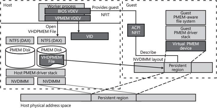
Figure 11-77 The virtual PM architecture.

A virtual PM device exposes a contiguous address space, virtualized from the host (this means that the host VHDPMEM files don’t not need to be contiguous). It supports both DAX and block mode, which, as in the host case, must be decided at volume-format time, and supports large and huge pages, which are leveraged in the same way as on the host system. Only generation 2 virtual machines support virtual PM devices and the mapping of VHDPMEM files.

Storage Spaces Direct in Windows Server 2019 also supports DAX disks in its virtual storage pools. One or more DAX disks can be part of an aggregated array of mixed-type disks. The PM disks in the array can be configured to provide the capacity or performance tier of a bigger tiered virtual disk or can be configured to act as a high-performance cache. More details on Storage Spaces are available later in this chapter.

EXPERIMENT: Create and mount a VHDPMEM image

As discussed in the previous paragraph, virtual PM disks can be created, converted, and assigned to a HyperV virtual machine using PowerShell. In this experiment, you need a DAX disk and a generation 2 virtual machine with Windows 10 October Update (RS5, or later releases) installed (describing how to create a VM is outside the scope of this experiment). Open an administrative Windows PowerShell prompt, move to your DAX-mode disk, and create the virtual PM disk (in the example, the DAX disk is located in the Q: drive):

Click here to view code image

PS Q:\> New-VHD VmPmemDis.vhdpmem -Fixed -SizeBytes 256GB -PhysicalSectorSizeBytes 4096
    
    ComputerName            : 37-4611k2635
    Path                    : Q:\VmPmemDis.vhdpmem
    VhdFormat               : VHDX
    VhdType                 : Fixed
    FileSize                : 274882101248
    Size                    : 274877906944
    MinimumSize             :
    LogicalSectorSize       : 4096
    PhysicalSectorSize      : 4096
    BlockSize               : 0
    ParentPath              :
    DiskIdentifier          : 3AA0017F-03AF-4948-80BE-B40B4AA6BE24
    FragmentationPercentage : 0
    Alignment               : 1
    Attached                : False
    DiskNumber              :
    IsPMEMCompatible        : True
    AddressAbstractionType  : None
    Number                  :

Virtual PM disks can be of fixed size only, meaning that all the space is allocated for the virtual disk—this is by design. The second step requires you to create the virtual PM controller and attach it to your virtual machine. Make sure that your VM is switched off, and type the following command. You should replace “TestPmVm” with the name of your virtual machine):

Click here to view code image

PS Q:\> Add-VMPmemController -VMName "TestPmVm"

Finally, you need to attach the created virtual PM disk to the virtual machine’s PM controller:

Click here to view code image

PS Q:\> Add-VMHardDiskDrive "TestVm" PMEM -ControllerLocation 1 -Path 'Q:\VmPmemDis.vhdpmem'

You can verify the result of the operation by using the Get-VMPmemController command:

Click here to view code image

PS Q:\> Get-VMPmemController -VMName "TestPmVm"
    
    VMName     ControllerNumber Drives
    ------     ---------------- ------
    TestPmVm   0                {Persistent Memory Device on PMEM controller number 0 at location 1}

If you switch on your virtual machine, you will find that Windows detects a new virtual disk. In the virtual machine, open the Disk Management MMC snap-in Tool (diskmgmt.msc) and initialize the disk using GPT partitioning. Then create a simple volume, assign a drive letter to it, but don’t format it.

You need to format the virtual PM disk in DAX mode. Open an administrative command prompt window in the virtual machine. Assuming that your virtual-pm disk drive letter is E:, you need to use the following command:

Click here to view code image

C:\>format e: /DAX /fs:NTFS /q
    The type of the file system is RAW.
    The new file system is NTFS.
    
    WARNING, ALL DATA ON NON-REMOVABLE DISK
    DRIVE E: WILL BE LOST!
    Proceed with Format (Y/N)? y
    QuickFormatting 256.0 GB
    Volume label (32 characters, ENTER for none)? DAX-In-Vm
    Creating file system structures.
    Format complete.
         256.0 GB total disk space.
         255.9 GB are available.

You can then confirm that the virtual disk has been formatted in DAX mode by using the fsutil.exe built-in tool, specifying the fsinfo volumeinfo command-line arguments:

Click here to view code image

C:\>fsutil fsinfo volumeinfo C:
    Volume Name : DAX-In-Vm
    Volume Serial Number : 0x1a1bdc32
    Max Component Length : 255
    File System Name : NTFS
    Is ReadWrite
    Not Thinly-Provisioned
    Supports Case-sensitive filenames
    Preserves Case of filenames
    Supports Unicode in filenames
    Preserves & Enforces ACL’s
    Supports Disk Quotas
    Supports Reparse Points
    Returns Handle Close Result Information
    Supports POSIX-style Unlink and Rename
    Supports Object Identifiers
    Supports Named Streams
    Supports Hard Links
    Supports Extended Attributes
    Supports Open By FileID
    Supports USN Journal
    Is DAX Volume

Resilient File System (ReFS)

The release of Windows Server 2012 R2 saw the introduction of a new advanced file system, the Resilient File System (also known as ReFS). This file system is part of a new storage architecture, called Storage Spaces, which, among other features, allows the creation of a tiered virtual volume composed of a solid-state drive and a classical rotational disk. (An introduction of Storage Spaces, and Tiered Storage, is presented later in this chapter). ReFS is a “write-to-new” file system, which means that file system metadata is never updated in place; updated metadata is written in a new place, and the old one is marked as deleted. This property is important and is one of the features that provides data integrity. The original goals of ReFS were the following:

1. Self-healing, online volume check and repair (providing close to zero unavailability due to file system corruption) and write-through support. (Write-through is discussed later in this section.)

2. Data integrity for all user data (hardware and software).

3. Efficient and fast file snapshots (block cloning).

4. Support for extremely large volumes (exabyte sizes) and files.

5. Automatic tiering of data and metadata, support for SMR (shingled magnetic recording) and future solid-state disks.

There have been different versions of ReFS. The one described in this book is referred to as ReFS v2, which was first implemented in Windows Server 2016. Figure 11-78 shows an overview of the different high-level implementations between NTFS and ReFS. Instead of completely rewriting the NTFS file system, ReFS uses another approach by dividing the implementation of NTFS into two parts: one part understands the on-disk format, and the other does not.

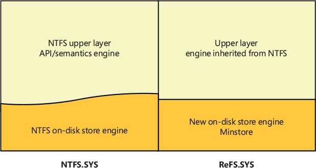
Figure 11-78 ReFS high-level implementation compared to NTFS.

ReFS replaces the on-disk storage engine with Minstore. Minstore is a recoverable object store library that provides a key-value table interface to its callers, implements allocate-on-write semantics for modification to those tables, and integrates with the Windows cache manager. Essentially, Minstore is a library that implements the core of a modern, scalable copy-on-write file system. Minstore is leveraged by ReFS to implement files, directories, and so on. Understanding the basics of Minstore is needed to describe ReFS, so let’s start with a description of Minstore.

Minstore architecture

Everything in Minstore is a table. A table is composed of multiple rows, which are made of a key-value pair. Minstore tables, when stored on disk, are represented using B+ trees. When kept in volatile memory (RAM), they are represented using hash tables. B+ trees, also known as balanced trees, have different important properties:

1. They usually have a large number of children per node.

2. They store data pointers (a pointer to the disk file block that contains the key value) only on the leaves—not on internal nodes.

3. Every path from the root node to a leaf node is of the same length.

Other file systems (like NTFS) generally use B-trees (another data structure that generalizes a binary search-tree, not to be confused with the term “Binary tree”) to store the data pointer, along with the key, in each node of the tree. This technique greatly reduces the number of entries that can be packed into a node of a B-tree, thereby contributing to the increase in the number of levels in the B-tree, hence increasing the search time of a record.

Figure 11-79 shows an example of B+ tree. In the tree shown in the figure, the root and the internal node contain only keys, which are used for properly accessing the data located in the leaf’s nodes. Leaf nodes are all at the same level and are generally linked together. As a consequence, there is no need to emit lots of I/O operations for finding an element in the tree.

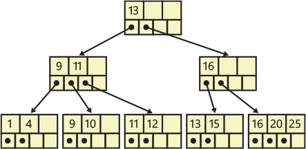
Figure 11-79 A sample B+ tree. Only the leaf nodes contain data pointers. Director nodes contain only links to children nodes.

For example, let’s assume that Minstore needs to access the node with the key 20. The root node contains one key used as an index. Keys with a value above or equal to 13 are stored in one of the children indexed by the right pointer; meanwhile, keys with a value less than 13 are stored in one of the left children. When Minstore has reached the leaf, which contains the actual data, it can easily access the data also for node with keys 16 and 25 without performing any full tree scan.

Furthermore, the leaf nodes are usually linked together using linked lists. This means that for huge trees, Minstore can, for example, query all the files in a folder by accessing the root and the intermediate nodes only once—assuming that in the figure all the files are represented by the values stored in the leaves. As mentioned above, Minstore generally uses a B+ tree for representing different objects than files or directories.

In this book, we use the term B+ tree and B+ table for expressing the same concept. Minstore defines different kind of tables. A table can be created, it can have rows added to it, deleted from it, or updated inside of it. An external entity can enumerate the table or find a single row. The Minstore core is represented by the object table. The object table is an index of the location of every root (nonembedded) B+ trees in the volume. B+ trees can be embedded within other trees; a child tree’s root is stored within the row of a parent tree.

Each table in Minstore is defined by a composite and a schema. A composite is just a set of rules that describe the behavior of the root node (sometimes even the children) and how to find and manipulate each node of the B+ table. Minstore supports two kinds of root nodes, managed by their respective composites:

• ■    Copy on Write (CoW): This kind of root node moves its location when the tree is modified. This means that in case of modification, a brand-new B+ tree is written while the old one is marked for deletion. In order to deal with these nodes, the corresponding composite needs to maintain an object ID that will be used when the table is written.

• ■    Embedded: This kind of root node is stored in the data portion (the value of a leaf node) of an index entry of another B+ tree. The embedded composite maintains a reference to the index entry that stores the embedded root node.

Specifying a schema when the table is created tells Minstore what type of key is being used, how big the root and the leaf nodes of the table should be, and how the rows in the table are laid out. ReFS uses different schemas for files and directories. Directories are B+ table objects referenced by the object table, which can contain three different kinds of rows (files, links, and file IDs). In ReFS, the key of each row represents the name of the file, link, or file ID. Files are tables that contain attributes in their rows (attribute code and value pairs).

Every operation that can be performed on a table (close, modify, write to disk, or delete) is represented by a Minstore transaction. A Minstore transaction is similar to a database transaction: a unit of work, sometimes made up of multiple operations, that can succeed or fail only in an atomic way. The way in which tables are written to the disk is through a process known as updating the tree. When a tree update is requested, transactions are drained from the tree, and no transactions are allowed to start until the update is finished.

One important concept used in ReFS is the embedded table: a B+ tree that has the root node located in a row of another B+ tree. ReFS uses embedded tables extensively. For example, every file is a B+ tree whose roots are embedded in the row of directories. Embedded tables also support a move operation that changes the parent table. The size of the root node is fixed and is taken from the table’s schema.

B+ tree physical layout

In Minstore, a B+ tree is made of buckets. Buckets are the Minstore equivalent of the general B+ tree nodes. Leaf buckets contain the data that the tree is storing; intermediate buckets are called director nodes and are used only for direct lookups to the next level in the tree. (In Figure 11-79, each node is a bucket.) Because director nodes are used only for directing traffic to child buckets, they need not have exact copies of a key in a child bucket but can instead pick a value between two buckets and use that. (In ReFS, usually the key is a compressed file name.) The data of an intermediate bucket instead contains both the logical cluster number (LCN) and a checksum of the bucket that it’s pointing to. (The checksum allows ReFS to implement self-healing features.) The intermediate nodes of a Minstore table could be considered as a Merkle tree, in which every leaf node is labelled with the hash of a data block, and every nonleaf node is labelled with the cryptographic hash of the labels of its child nodes.

Every bucket is composed of an index header that describes the bucket, and a footer, which is an array of offsets pointing to the index entries in the correct order. Between the header and the footer there are the index entries. An index entry represents a row in the B+ table; a row is a simple data structure that gives the location and size of both the key and data (which both reside in the same bucket). Figure 11-80 shows an example of a leaf bucket containing three rows, indexed by the offsets located in the footer. In leaf pages, each row contains the key and the actual data (or the root node of another embedded tree).

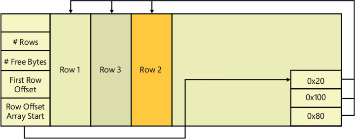
Figure 11-80 A leaf bucket with three index entries that are ordered by the array of offsets in the footer.

Allocators

When the file system asks Minstore to allocate a bucket (the B+ table requests a bucket with a process called pinning the bucket), the latter needs a way to keep track of the free space of the underlaying medium. The first version of Minstore used a hierarchical allocator, which meant that there were multiple allocator objects, each of which allocated space out of its parent allocator. When the root allocator mapped the entire space of the volume, each allocator became a B+ tree that used the lcn-count table schema. This schema describes the row’s key as a range of LCN that the allocator has taken from its parent node, and the row’s value as an allocator region. In the original implementation, an allocator region described the state of each chunk in the region in relation to its children nodes: free or allocated and the owner ID of the object that owns it.

Figure 11-81 shows a simplified version of the original implementation of the hierarchical allocator. In the picture, a large allocator has only one allocation unit set: the space represented by the bit has been allocated for the medium allocator, which is currently empty. In this case, the medium allocator is a child of the large allocator.

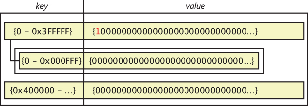
Figure 11-81 The old hierarchical allocator.

B+ tables deeply rely on allocators to get new buckets and to find space for the copy-on-write copies of existing buckets (implementing the write-to-new strategy). The latest Minstore version replaced the hierarchical allocator with a policy-driven allocator, with the goal of supporting a central location in the file system that would be able to support tiering. A tier is a type of the storage device—for example, an SSD, NVMe, or classical rotational disk. Tiering is discussed later in this chapter. It is basically the ability to support a disk composed of a fast random-access zone, which is usually smaller than the slow sequential-only area.

The new policy-driven allocator is an optimized version (supporting a very large number of allocations per second) that defines different allocation areas based on the requested tier (the type of underlying storage device). When the file system requests space for new data, the central allocator decides which area to allocate from by a policy-driven engine. This policy engine is tiering-aware (this means that metadata is always written to the performance tiers and never to SMR capacity tiers, due to the random-write nature of the metadata), supports ReFS bands, and implements deferred allocation logic (DAL). The deferred allocation logic relies on the fact that when the file system creates a file, it usually also allocates the needed space for the file content. Minstore, instead of returning to the underlying file system an LCN range, returns a token containing the space reservation that provides a guarantee against the disk becoming full. When the file is ultimately written, the allocator assigns LCNs for the file’s content and updates the metadata. This solves problems with SMR disks (which are covered later in this chapter) and allows ReFS to be able to create even huge files (64 TB or more) in less than a second.

The policy-driven allocator is composed of three central allocators, implemented on-disk as global B+ tables. When they’re loaded in memory, the allocators are represented using AVL trees, though. An AVL tree is another kind of self-balancing binary tree that’s not covered in this book. Although each row in the B+ table is still indexed by a range, the data part of the row could contain a bitmap or, as an optimization, only the number of allocated clusters (in case the allocated space is contiguous). The three allocators are used for different purposes:

• ■    The Medium Allocator (MAA) is the allocator for each file in the namespace, except for some B+ tables allocated from the other allocators. The Medium Allocator is a B+ table itself, so it needs to find space for its metadata updates (which still follow the write-to-new strategy). This is the role of the Small Allocator (SAA).

• ■    The Small Allocator (SAA) allocates space for itself, for the Medium Allocator, and for two tables: the Integrity State table (which allows ReFS to support Integrity Streams) and the Block Reference Counter table (which allows ReFS to support a file’s block cloning).

• ■    The Container Allocator (CAA) is used when allocating space for the container table, a fundamental table that provides cluster virtualization to ReFS and is also deeply used for container compaction. (See the following sections for more details.) Furthermore, the Container Allocator contains one or more entries for describing the space used by itself.

When the Format tool initially creates the basic data structures for ReFS, it creates the three allocators. The Medium Allocator initially describes all the volume’s clusters. Space for the SAA and CAA metadata (which are B+ tables) is allocated from the MAA (this is the only time that ever happens in the volume lifetime). An entry for describing the space used by the Medium Allocator is inserted in the SAA. Once the allocators are created, additional entries for the SAA and CAA are no longer allocated from the Medium Allocator (except in case ReFS finds corruption in the allocators themselves).

To perform a write-to-new operation for a file, ReFS must first consult the MAA allocator to find space for the write to go to. In a tiered configuration, it does so with awareness of the tiers. Upon successful completion, it updates the file’s stream extent table to reflect the new location of that extent and updates the file’s metadata. The new B+ tree is then written to the disk in the free space block, and the old table is converted as free space. If the write is tagged as a write-through, meaning that the write must be discoverable after a crash, ReFS writes a log record for recording the write-to-new operation. (See the “ReFS write-through” section later in this chapter for further details).

Page table

When Minstore updates a bucket in the B+ tree (maybe because it needs to move a child node or even add a row in the table), it generally needs to update the parent (or director) nodes. (More precisely, Minstore uses different links that point to a new and an old child bucket for every node.) This is because, as we have described earlier, every director node contains the checksum of its leaves. Furthermore, the leaf node could have been moved or could even have been deleted. This leads to synchronization problems; for example, imagine a thread that is reading the B+ tree while a row is being deleted. Locking the tree and writing every modification on the physical medium would be prohibitively expensive. Minstore needs a convenient and fast way to keep track of the information about the tree. The Minstore Page Table (unrelated to the CPU’s page table), is an in-memory hash table private to each Minstore’s root table—usually the directory and file table—which keeps track of which bucket is dirty, freed, or deleted. This table will never be stored on the disk. In Minstore, the terms bucket and page are used interchangeably; a page usually resides in memory, whereas a bucket is stored on disk, but they express exactly the same high-level concept. Trees and tables also are used interchangeably, which explains why the page table is called as it is. The rows of a page table are composed of the LCN of the target bucket, as a Key, and a data structure that keeps track of the page states and assists the synchronization of the B+ tree as a value.

When a page is first read or created, a new entry will be inserted into the hash table that represents the page table. An entry into the page table can be deleted only if all the following conditions are met:

• ■    There are no active transactions accessing the page.

• ■    The page is clean and has no modifications.

• ■    The page is not a copy-on-write new page of a previous one.

Thanks to these rules, clean pages usually come into the page table and are deleted from it repeatedly, whereas a page that is dirty would stay in the page table until the B+ tree is updated and finally written to disk. The process of writing the tree to stable media depends heavily upon the state in the page table at any given time. As you can see from Figure 11-82, the page table is used by Minstore as an in-memory cache, producing an implicit state machine that describes each state of a page.

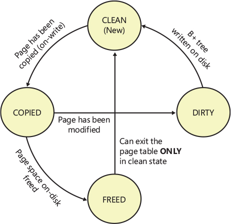
Figure 11-82 The diagram shows the states of a dirty page (bucket) in the page table. A new page is produced due to copy-on-write of an old page or if the B+ tree is growing and needs more space for storing the bucket.

Minstore I/O

In Minstore, reads and writes to the B+ tree in the final physical medium are performed in a different way: tree reads usually happen in portions, meaning that the read operation might only include some leaf buckets, for example, and occurs as part of transactional access or as a preemptive prefetch action. After a bucket is read into the cache (see the “Cache manager” section earlier in this chapter), Minstore still can’t interpret its data because the bucket checksum needs to be verified. The expected checksum is stored in the parent node: when the ReFS driver (which resides above Minstore) intercepts the read data, it knows that the node still needs to be validated: the parent node is already in the cache (the tree has been already navigated for reaching the child) and contains the checksum of the child. Minstore has all the needed information for verifying that the bucket contains valid data. Note that there could be pages in the page table that have been never accessed. This is because their checksum still needs to be validated.

Minstore performs tree updates by writing the entire B+ tree as a single transaction. The tree update process writes dirty pages of the B+ tree to the physical disk. There are multiple reasons behind a tree update—an application explicitly flushing its changes, the system running in low memory or similar conditions, the cache manager flushing cached data to disk, and so on. It’s worth mentioning that Minstore usually writes the new updated trees lazily with the lazy writer thread. As seen in the previous section, there are several triggers to kick in the lazy writer (for example, when the number of the dirty pages reaches a certain threshold).

Minstore is unaware of the actual reason behind the tree update request. The first thing that Minstore does is make sure that no other transactions are modifying the tree (using complex synchronization primitives). After initial synchronization, it starts to write dirty pages and with old deleted pages. In a write-to-new implementation, a new page represents a bucket that has been modified and its content replaced; a freed page is an old page that needs to be unlinked from the parent. If a transaction wants to modify a leaf node, it copies (in memory) the root bucket and the leaf page; Minstore then creates the corresponding page table entries in the page table without modifying any link.

The tree update algorithm enumerates each page in the page table. However, the page table has no concept of which level in the B+ tree the page resides, so the algorithm checks even the B+ tree by starting from the more external node (usually the leaf), up to the root nodes. For each page, the algorithm performs the following steps:

1. Checks the state of the page. If it’s a freed page, it skips the page. If it’s a dirty page, it updates its parent pointer and checksum and puts the page in an internal list of pages to write.

2. Discards the old page.

When the algorithm reaches the root node, it updates its parent pointer and checksum directly in the object table and finally puts also the root bucket in the list of pages to write. Minstore is now able to write the new tree in the free space of the underlying volume, preserving the old tree in its original location. The old tree is only marked as freed but is still present in the physical medium. This is an important characteristic that summarizes the write-to-new strategy and allows the ReFS file system (which resides above Minstore) to support advanced online recovery features. Figure 11-83 shows an example of the tree update process for a B+ table that contains two new leaf pages (A’ and B’). In the figure, pages located in the page table are represented in a lighter shade, whereas the old pages are shown in a darker shade.

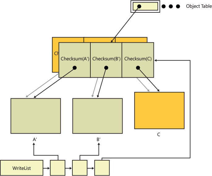
Figure 11-83 Minstore tree update process.

Maintaining exclusive access to the tree while performing the tree update can represent a performance issue; no one else can read or write from a B+ tree that has been exclusively locked. In the latest versions of Windows 10, B+ trees in Minstore became generational—a generation number is attached to each B+ tree. This means that a page in the tree can be dirty with regard to a specific generation. If a page is originally dirty for only a specific tree generation, it can be directly updated, with no need to copy-on-write because the final tree has still not been written to disk.

In the new model, the tree update process is usually split in two phases:

• ■    Failable phase: Minstore acquires the exclusive lock on the tree, increments the tree’s generation number, calculates and allocates the needed memory for the tree update, and finally drops the lock to shared.

• ■    Nonfailable phase: This phase is executed with a shared lock (meaning that other I/O can read from the tree), Minstore updates the links of the director nodes and all the tree’s checksums, and finally writes the final tree to the underlying disk. If another transaction wants to modify the tree while it’s being written to disk, it detects that the tree’s generation number is higher, so it copy-on-writes the tree again.

With the new schema, Minstore holds the exclusive lock only in the failable phase. This means that tree updates can run in parallel with other Minstore transactions, significantly improving the overall performance.

ReFS architecture

As already introduced in previous paragraphs, ReFS (the Resilient file system) is a hybrid of the NTFS implementation and Minstore, where every file and directory is a B+ tree configured by a particular schema. The file system volume is a flat namespace of directories. As discussed previously, NTFS is composed of different components:

• ■    Core FS support: Describes the interface between the file system and other system components, like the cache manager and the I/O subsystem, and exposes the concept of file create, open, read, write, close, and so on.

• ■    High-level FS feature support: Describes the high-level features of a modern file system, like file compression, file links, quota tracking, reparse points, file encryption, recovery support, and so on.

• ■    On-disk dependent components and data structures MFT and file records, clusters, index package, resident and nonresident attributes, and so on (see the “The NT file system (NTFS)” section earlier in this chapter for more details).

ReFS keeps the first two parts largely unchanged and replaces the rest of the on-disk dependent components with Minstore, as shown in Figure 11-84.

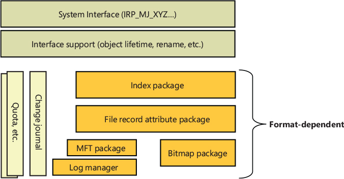
Figure 11-84 ReFS architecture’s scheme.

In the “NTFS driver” section of this chapter, we introduced the entities that link a file handle to the file system’s on-disk structure. In the ReFS file system driver, those data structures (the stream control block, which represents the NTFS attribute that the caller is trying to read, and the file control block, which contains a pointer to the file record in the disk’s MFT) are still valid, but have a slightly different meaning in respect to their underlying durable storage. The changes made to these objects go through Minstore instead of being directly translated in changes to the on-disk MFT. As shown in Figure 11-85, in ReFS:

• ■    A file control block (FCB) represents a single file or directory and, as such, contains a pointer to the Minstore B+ tree, a reference to the parent directory’s stream control block and key (the directory name). The FCB is pointed to by the file object, through the FsContext2 field.

• ■    A stream control block (SCB) represents an opened stream of the file object. The data structure used in ReFS is a simplified version of the NTFS one. When the SCB represents directories, though, the SCB has a link to the directory’s index, which is located in the B+ tree that represents the directory. The SCB is pointed to by the file object, through the FsContext field.

• ■    A volume control block (VCB) represents a currently mounted volume, formatted by ReFS. When a properly formatted volume has been identified by the ReFS driver, a VCB data structure is created, attached into the volume device object extension, and linked into a list located in a global data structure that the ReFS file system driver allocates at its initialization time. The VCB contains a table of all the directory FCBs that the volume has currently opened, indexed by their reference ID.

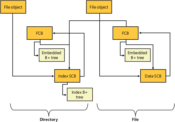
Figure 11-85 ReFS files and directories in-memory data structures.

In ReFS, every open file has a single FCB in memory that can be pointed to by different SCBs (depending on the number of streams opened). Unlike NTFS, where the FCB needs only to know the MFT entry of the file to correctly change an attribute, the FCB in ReFS needs to point to the B+ tree that represents the file record. Each row in the file’s B+ tree represents an attribute of the file, like the ID, full name, extents table, and so on. The key of each row is the attribute code (an integer value).

File records are entries in the directory in which files reside. The root node of the B+ tree that represents a file is embedded into the directory entry’s value data and never appears in the object table. The file data streams, which are represented by the extents table, are embedded B+ trees in the file record. The extents table is indexed by range. This means that every row in the extent table has a VCN range used as the row’s key, and the LCN of the file’s extent used as the row’s value. In ReFS, the extents table could become very large (it is indeed a regular B+ tree). This allows ReFS to support huge files, bypassing the limitations of NTFS.

Figure 11-86 shows the object table, files, directories, and the file extent table, which in ReFS are all represented through B+ trees and provide the file system namespace.

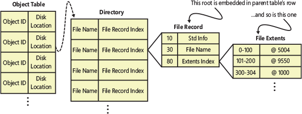
Figure 11-86 Files and directories in ReFS.

Directories are Minstore B+ trees that are responsible for the single, flat namespace. A ReFS directory can contain:

• ■    Files

• ■    Links to directories

• ■    Links to other files (file IDs)

Rows in the directory B+ tree are composed of a <key, <type, value>> pair, where the key is the entry’s name and the value depends on the type of directory entry. With the goal of supporting queries and other high-level semantics, Minstore also stores some internal data in invisible directory rows. These kinds of rows have have their key starting with a Unicode zero character. Another row that is worth mentioning is the directory’s file row. Every directory has a record, and in ReFS that file record is stored as a file row in the self-same directory, using a well-known zero key. This has some effect on the in-memory data structures that ReFS maintains for directories. In NTFS, a directory is really a property of a file record (through the Index Root and Index Allocation attributes); in ReFS, a directory is a file record stored in the directory itself (called directory index record). Therefore, whenever ReFS manipulates or inspects files in a directory, it must ensure that the directory index is open and resident in memory. To be able to update the directory, ReFS stores a pointer to the directory’s index record in the opened stream control block.

The described configuration of the ReFS B+ trees does not solve an important problem. Every time the system wants to enumerate the files in a directory, it needs to open and parse the B+ tree of each file. This means that a lot of I/O requests to different locations in the underlying medium are needed. If the medium is a rotational disk, the performance would be rather bad.

To solve the issue, ReFS stores a STANDARD_INFORMATION data structure in the root node of the file’s embedded table (instead of storing it in a row of the child file’s B+ table). The STANDARD _INFORMATION data includes all the information needed for the enumeration of a file (like the file’s access time, size, attributes, security descriptor ID, the update sequence number, and so on). A file’s embedded root node is stored in a leaf bucket of the parent directory’s B+ tree. By having the data structure located in the file’s embedded root node, when the system enumerates files in a directory, it only needs to parse entries in the directory B+ tree without accessing any B+ tables describing individual files. The B+ tree that represents the directory is already in the page table, so the enumeration is quite fast.

ReFS on-disk structure

This section describes the on-disk structure of a ReFS volume, similar to the previous NTFS section. The section focuses on the differences between NTFS and ReFS and will not cover the concepts already described in the previous section.

The Boot sector of a ReFS volume consists of a small data structure that, similar to NTFS, contains basic volume information (serial number, cluster size, and so on), the file system identifier (the ReFS OEM string and version), and the ReFS container size (more details are covered in the “Shingled magnetic recording (SMR) volumes” section later in the chapter). The most important data structure in the volume is the volume super block. It contains the offset of the latest volume checkpoint records and is replicated in three different clusters. ReFS, to be able to mount a volume, reads one of the volume checkpoints, verifies and parses it (the checkpoint record includes a checksum), and finally gets the offset of each global table.

The volume mounting process opens the object table and gets the needed information for reading the root directory, which contains all of the directory trees that compose the volume namespace. The object table, together with the container table, is indeed one of the most critical data structures that is the starting point for all volume metadata. The container table exposes the virtualization namespace, so without it, ReFS would not able to correctly identify the final location of any cluster. Minstore optionally allows clients to store information within its object table rows. The object table row values, as shown in Figure 11-87, have two distinct parts: a portion owned by Minstore and a portion owned by ReFS. ReFS stores parent information as well as a high watermark for USN numbers within a directory (see the section “Security and change journal” later in this chapter for more details).

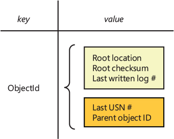
Figure 11-87 The object table entry composed of a ReFS part (bottom rectangle) and Minstore part (top rectangle).

Object IDs

Another problem that ReFS needs to solve regards file IDs. For various reasons—primarily for tracking and storing metadata about files in an efficient way without tying information to the namespace—ReFS needs to support applications that open a file through their file ID (using the OpenFileById API, for example). NTFS accomplishes this through the $Extend\$ObjId file (using the $0 index root attribute; see the previous NTFS section for more details). In ReFS, assigning an ID to every directory is trivial; indeed, Minstore stores the object ID of a directory in the object table. The problem arises when the system needs to be able to assign an ID to a file; ReFS doesn’t have a central file ID repository like NTFS does. To properly find a file ID located in a directory tree, ReFS splits the file ID space into two portions: the directory and the file. The directory ID consumes the directory portion and is indexed into the key of an object table’s row. The file portion is assigned out of the directory’s internal file ID space. An ID that represents a directory usually has a zero in its file portion, but all files inside the directory share the same directory portion. ReFS supports the concept of file IDs by adding a separate row (composed of a <FileId, FileName> pair) in the directory’s B+ tree, which maps the file ID to the file name within the directory.

When the system is required to open a file located in a ReFS volume using its file ID, ReFS satisfies the request by:

1. Opening the directory specified by the directory portion

2. Querying the FileId row in the directory B+ tree that has the key corresponding to the file portion

3. Querying the directory B+ tree for the file name found in the last lookup.

Careful readers may have noted that the algorithm does not explain what happens when a file is renamed or moved. The ID of a renamed file should be the same as its previous location, even if the ID of the new directory is different in the directory portion of the file ID. ReFS solves the problem by replacing the original file ID entry, located in the old directory B+ tree, with a new “tombstone” entry, which, instead of specifying the target file name in its value, contains the new assigned ID of the renamed file (with both the directory and the file portion changed). Another new File ID entry is also allocated in the new directory B+ tree, which allows assigning the new local file ID to the renamed file. If the file is then moved to yet another directory, the second directory has its ID entry deleted because it’s no longer needed; one tombstone, at most, is present for any given file.

Security and change journal

The mechanics of supporting Windows object security in the file system lie mostly in the higher components that are implemented by the portions of the file system remained unchanged since NTFS. The underlying on-disk implementation has been changed to support the same set of semantics. In ReFS, object security descriptors are stored in the volume’s global security directory B+ table. A hash is computed for every security descriptor in the table (using a proprietary algorithm, which operates only on self-relative security descriptors), and an ID is assigned to each.

When the system attaches a new security descriptor to a file, the ReFS driver calculates the security descriptor’s hash and checks whether it’s already present in the global security table. If the hash is present in the table, ReFS resolves its ID and stores it in the STANDARD_INFORMATION data structure located in the embedded root node of the file’s B+ tree. In case the hash does not already exist in the global security table, ReFS executes a similar procedure but first adds the new security descriptor in the global B+ tree and generates its new ID.

The rows of the global security table are of the format <<hash, ID>, <security descriptor, ref. count>>, where the hash and the ID are as described earlier, the security descriptor is the raw byte payload of the security descriptor itself, and ref. count is a rough estimate of how many objects on the volume are using the security descriptor.

As described in the previous section, NTFS implements a change journal feature, which provides applications and services with the ability to query past changes to files within a volume. ReFS implements an NTFS-compatible change journal implemented in a slightly different way. The ReFS journal stores change entries in the change journal file located in another volume’s global Minstore B+ tree, the metadata directory table. ReFS opens and parses the volume’s change journal file only once the volume is mounted. The maximum size of the journal is stored in the $USN_MAX attribute of the journal file. In ReFS, each file and directory contains its last USN (update sequence number) in the STANDARD_INFORMATION data structure stored in the embedded root node of the parent directory. Through the journal file and the USN number of each file and directory, ReFS can provide the three FSCTL used for reading and enumerate the volume journal file:

• ■    FSCTL_READ_USN_JOURNAL: Reads the USN journal directly. Callers specify the journal ID they’re reading and the number of the USN record they expect to read.

• ■    FSCTL_READ_FILE_USN_DATA: Retrieves the USN change journal information for the specified file or directory.

• ■    FSCTL_ENUM_USN_DATA: Scans all the file records and enumerates only those that have last updated the USN journal with a USN record whose USN is within the range specified by the caller. ReFS can satisfy the query by scanning the object table, then scanning each directory referred to by the object table, and returning the files in those directories that fall within the timeline specified. This is slow because each directory needs to be opened, examined, and so on. (Directories’ B+ trees can be spread across the disk.) The way ReFS optimizes this is that it stores the highest USN of all files in a directory in that directory’s object table entry. This way, ReFS can satisfy this query by visiting only directories it knows are within the range specified.

ReFS advanced features

In this section, we describe the advanced features of ReFS, which explain why the ReFS file system is a better fit for large server systems like the ones used in the infrastructure that provides the Azure cloud.

File’s block cloning (snapshot support) and sparse VDL

Traditionally, storage systems implement snapshot and clone functionality at the volume level (see dynamic volumes, for example). In modern datacenters, when hundreds of virtual machines run and are stored on a unique volume, such techniques are no longer able to scale. One of the original goals of the ReFS design was to support file-level snapshots and scalable cloning support (a VM typically maps to one or a few files in the underlying host storage), which meant that ReFS needed to provide a fast method to clone an entire file or even only chunks of it. Cloning a range of blocks from one file into a range of another file allows not only file-level snapshots but also finer-grained cloning for applications that need to shuffle blocks within one or more files. VHD diff-disk merge is one example.

ReFS exposes the new FSCTL_DUPLICATE_EXTENTS_TO_FILE to duplicate a range of blocks from one file into another range of the same file or to a different file. Subsequent to the clone operation, writes into cloned ranges of either file will proceed in a write-to-new fashion, preserving the cloned block. When there is only one remaining reference, the block can be written in place. The source and target file handle, and all the details from which the block should be cloned, which blocks to clone from the source, and the target range are provided as parameters.

As already seen in the previous section, ReFS indexes the LCNs that make up the file’s data stream into the extent index table, an embedded B+ tree located in a row of the file record. To support block cloning, Minstore uses a new global index B+ tree (called the block count reference table) that tracks the reference counts of every extent of blocks that are currently cloned. The index starts out empty. The first successful clone operation adds one or more rows to the table, indicating that the blocks now have a reference count of two. If one of the views of those blocks were to be deleted, the rows would be removed. This index is consulted in write operations to determine if write-to-new is required or if write-in-place can proceed. It’s also consulted before marking free blocks in the allocator. When freeing clusters that belong to a file, the reference counts of the cluster-range is decremented. If the reference count in the table reaches zero, the space is actually marked as freed.

Figure 11-88 shows an example of file cloning. After cloning an entire file (File 1 and File 2 in the picture), both files have identical extent tables, and the Minstore block count reference table shows two references to both volume extents.

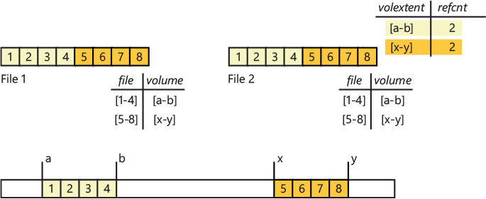
Figure 11-88 Cloning an ReFS file.

Minstore automatically merges rows in the block reference count table whenever possible with the intention of reducing the size of the table. In Windows Server 2016, HyperV makes use of the new cloning FSCTL. As a result, the duplication of a VM, and the merging of its multiple snapshots, is extremely fast.

ReFS supports the concept of a file Valid Data Length (VDL), in a similar way to NTFS. Using the $$ZeroRangeInStream file data stream, ReFS keeps track of the valid or invalid state for each allocated file’s data block. All the new allocations requested to the file are in an invalid state; the first write to the file makes the allocation valid. ReFS returns zeroed content to read requests from invalid file ranges. The technique is similar to the DAL, which we explained earlier in this chapter. Applications can logically zero a portion of file without actually writing any data using the FSCTL_SET_ZERO_DATA file system control code (the feature is used by HyperV to create fixed-size VHDs very quickly).

EXPERIMENT: Witnessing ReFS snapshot support through HyperV

In this experiment, you’re going to use HyperV for testing the volume snapshot support of ReFS. Using the HyperV manager, you need to create a virtual machine and install any operating system on it. At the first boot, take a checkpoint on the VM by right-clicking the virtual machine name and selecting the Checkpoint menu item. Then, install some applications on the virtual machine (the example below shows a Windows Server 2012 machine with Office installed) and take another checkpoint.

If you turn off the virtual machine and, using File Explorer, locate where the virtual hard disk file resides, you will find the virtual hard disk and multiple other files that represent the differential content between the current checkpoint and the previous one.

If you open the HyperV Manager again and delete the entire checkpoint tree (by right-clicking the first root checkpoint and selecting the Delete Checkpoint Subtree menu item), you will find that the entire merge process takes only a few seconds. This is explained by the fact that HyperV uses the block-cloning support of ReFS, through the FSCTL_DUPLICATE_EXTENTS_TO_FILE I/O control code, to properly merge the checkpoints’ content into the base virtual hard disk file. As explained in the previous paragraphs, block cloning doesn’t actually move any data. If you repeat the same experiment with a volume formatted using an exFAT or NTFS file system, you will find that the time needed to merge the checkpoints is much larger.

ReFS write-through

One of the goals of ReFS was to provide close to zero unavailability due to file system corruption. In the next section, we describe all of the available online repair methods that ReFS employs to recover from disk damage. Before describing them, it’s necessary to understand how ReFS implements write-through when it writes the transactions to the underlying medium.

The term write-through refers to any primitive modifying operation (for example, create file, extend file, or write block) that must not complete until the system has made a reasonable guarantee that the results of the operation will be visible after crash recovery. Write-through performance is critical for different I/O scenarios, which can be broken into two kinds of file system operations: data and metadata.

When ReFS performs an update-in-place to a file without requiring any metadata mutation (like when the system modifies the content of an already-allocated file, without extending its length), the write-through performance has minimal overhead. Because ReFS uses allocate-on-write for metadata, it’s expensive to give write-through guarantees for other scenarios when metadata change. For example, ensuring that a file has been renamed implies that the metadata blocks from the root of the file system down to the block describing the file’s name must be written to a new location. The allocate-on-write nature of ReFS has the property that it does not modify data in place. One implication of this is that recovery of the system should never have to undo any operations, in contrast to NTFS.

To achieve write-through, Minstore uses write-ahead-logging (or WAL). In this scheme, shown in Figure 11-89, the system appends records to a log that is logically infinitely long; upon recovery, the log is read and replayed. Minstore maintains a log of logical redo transaction records for all tables except the allocator table. Each log record describes an entire transaction, which has to be replayed at recovery time. Each transaction record has one or more operation redo records that describe the actual high-level operation to perform (such as insert [key K / value V] pair in Table X). The transaction record allows recovery to separate transactions and is the unit of atomicity (no transactions will be partially redone). Logically, logging is owned by every ReFS transaction; a small log buffer contains the log record. If the transaction is committed, the log buffer is appended to the in-memory volume log, which will be written to disk later; otherwise, if the transaction aborts, the internal log buffer will be discarded. Write-through transactions wait for confirmation from the log engine that the log has committed up until that point, while non-write-through transactions are free to continue without confirmation.

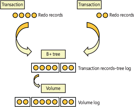
Figure 11-89 Scheme of Minstore’s write-ahead logging.

Furthermore, ReFS makes use of checkpoints to commit some views of the system to the underlying disk, consequently rendering some of the previously written log records unnecessary. A transaction’s redo log records no longer need to be redone once a checkpoint commits a view of the affected trees to disk. This implies that the checkpoint will be responsible for determining the range of log records that can be discarded by the log engine.

ReFS recovery support

To properly keep the file system volume available at all times, ReFS uses different recovery strategies. While NTFS has similar recovery support, the goal of ReFS is to get rid of any offline check disk utilities (like the Chkdsk tool used by NTFS) that can take many hours to execute in huge disks and require the operating system to be rebooted. There are mainly four ReFS recovery strategies:

• ■    Metadata corruption is detected via checksums and error-correcting codes. Integrity streams validate and maintain the integrity of the file’s data using a checksum of the file’s actual content (the checksum is stored in a row of the file’s B+ tree table), which maintains the integrity of the file itself and not only on its file-system metadata.

• ■    ReFS intelligently repairs any data that is found to be corrupt, as long as another valid copy is available. Other copies might be provided by ReFS itself (which keeps additional copies of its own metadata for critical structures such as the object table) or through the volume redundancy provided by Storage Spaces (see the “Storage Spaces” section later in this chapter).

• ■    ReFS implements the salvage operation, which removes corrupted data from the file system namespace while it’s online.

• ■    ReFS rebuilds lost metadata via best-effort techniques.

The first and second strategies are properties of the Minstore library on which ReFS depends (more details about the integrity streams are provided later in this section). The object table and all the global Minstore B+ tree tables contain a checksum for each link that points to the child (or director) nodes stored in different disk blocks. When Minstore detects that a block is not what it expects, it automatically attempts repair from one of its duplicated copies (if available). If the copy is not available, Minstore returns an error to the ReFS upper layer. ReFS responds to the error by initializing online salvage.

The term salvage refers to any fixes needed to restore as much data as possible when ReFS detects metadata corruption in a directory B+ tree. Salvage is the evolution of the zap technique. The goal of the zap was to bring back the volume online, even if this could lead to the loss of corrupted data. The technique removed all the corrupted metadata from the file namespace, which then became available after the repair.

Assume that a director node of a directory B+ tree becomes corrupted. In this case, the zap operation will fix the parent node, rewriting all the links to the child and rebalancing the tree, but the data originally pointed by the corrupted node will be completely lost. Minstore has no idea how to recover the entries addressed by the corrupted director node.

To solve this problem and properly restore the directory tree in the salvage process, ReFS needs to know subdirectories’ identifiers, even when the directory table itself is not accessible (because it has a corrupted director node, for example). Restoring part of the lost directory tree is made possible by the introduction of a volume global table, called called the parent-child table, which provides a directory’s information redundancy.

A key in the parent–child table represents the parent table’s ID, and the data contains a list of child table IDs. Salvage scans this table, reads the child tables list, and re-creates a new non-corrupted B+ tree that contains all the subdirectories of the corrupted node. In addition to needing child table IDs, to completely restore the corrupted parent directory, ReFS still needs the name of the child tables, which were originally stored in the keys of the parent B+ tree. The child table has a self-record entry with this information (of type link to directory; see the previous section for more details). The salvage process opens the recovered child table, reads the self-record, and reinserts the directory link into the parent table. The strategy allows ReFS to recover all the subdirectories of a corrupted director or root node (but still not the files). Figure 11-90 shows an example of zap and salvage operations on a corrupted root node representing the Bar directory. With the salvage operation, ReFS is able to quickly bring the file system back online and loses only two files in the directory.

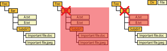
Figure 11-90 Comparison between the zap and salvage operations.

The ReFS file system, after salvage completes, tries to rebuild missing information using various best-effort techniques; for example, it can recover missing file IDs by reading the information from other buckets (thanks to the collating rule that separates files’ IDs and tables). Furthermore, ReFS also augments the Minstore object table with a little bit of extra information to expedite repair. Although ReFS has these best-effort heuristics, it’s important to understand that ReFS primarily relies on the redundancy provided by metadata and the storage stack in order to repair corruption without data loss.

In the very rare cases in which critical metadata is corrupted, ReFS can mount the volume in read-only mode, but not for any corrupted tables. For example, in case that the container table and all of its duplicates would all be corrupted, the volume wouldn’t be mountable in read-only mode. By skipping over these tables, the file system can simply ignore the usage of such global tables (like the allocator, for example), while still maintaining a chance for the user to recover her data.

Finally, ReFS also supports file integrity streams, where a checksum is used to guarantee the integrity of a file’s data (and not only of the file system’s metadata). For integrity streams, ReFS stores the checksum of each run that composes the file’s extent table (the checksum is stored in the data section of an extent table’s row). The checksum allows ReFS to validate the integrity of the data before accessing it. Before returning any data that has integrity streams enabled, ReFS will first calculate its checksum and compares it to the checksum contained in the file metadata. If the checksums don’t match, then the data is corrupt.

The ReFS file system exposes the FSCTL_SCRUB_DATA control code, which is used by the scrubber (also known as the data integrity scanner). The data integrity scanner is implemented in the Discan.dll library and is exposed as a task scheduler task, which executes at system startup and every week. When the scrubber sends the FSCTL to the ReFS driver, the latter starts an integrity check of the entire volume: the ReFS driver checks the boot section, each global B+ tree, and file system’s metadata.

Note

The online Salvage operation, described in this section, is different from its offline counterpart. The refsutil.exe tool, which is included in Windows, supports this operation. The tool is used when the volume is so corrupted that it is not even mountable in read-only mode (a rare condition). The offline Salvage operation navigates through all the volume clusters, looking for what appears to be metadata pages, and uses best-effort techniques to assemble them back together.

Leak detection

A cluster leak describes the situation in which a cluster is marked as allocated, but there are no references to it. In ReFS, cluster leaks can happen for different reasons. When a corruption is detected on a directory, online salvage is able to isolate the corruption and rebuild the tree, eventually losing only some files that were located in the root directory itself. A system crash before the tree update algorithm has written a Minstore transaction to disk can lead to a file name getting lost. In this case, the file’s data is correctly written to disk, but ReFS has no metadata that point to it. The B+ tree table representing the file itself can still exist somewhere in the disk, but its embedded table is no longer linked in any directory B+ tree.

The built-in refsutil.exe tool available in Windows supports the Leak Detection operation, which can scan the entire volume and, using Minstore, navigate through the entire volume namespace. It then builds a list of every B+ tree found in the namespace (every tree is identified by a well-known data structure that contains an identification header), and, by querying the Minstore allocators, compares the list of each identified tree with the list of trees that have been marked valid by the allocator. If it finds a discrepancy, the leak detection tool notifies the ReFS file system driver, which will mark the clusters allocated for the found leaked tree as freed.

Another kind of leak that can happen on the volume affects the block reference counter table, such as when a cluster’s range located in one of its rows has a higher reference counter number than the actual files that reference it. The lower-case tool is able to count the correct number of references and fix the problem.

To correctly identify and fix leaks, the leak detection tool must operate on an offline volume, but, using a similar technique to NTFS’ online scan, it can operate on a read-only snapshot of the target volume, which is provided by the Volume Shadow Copy service.

EXPERIMENT: Use Refsutil to find and fix leaks on a ReFS volume

In this experiment, you use the built-in refsutil.exe tool on a ReFS volume to find and fix cluster leaks that could happen on a ReFS volume. By default, the tool doesn’t require a volume to be unmounted because it operates on a read-only volume snapshot. To let the tool fix the found leaks, you can override the setting by using the /x command-line argument. Open an administrative command prompt and type the following command. (In the example, a 1 TB ReFS volume was mounted as the E: drive. The /v switch enables the tool’s verbose output.)

Click here to view code image

C:\>refsutil leak /v e:
    Creating volume snapshot on drive \\?\Volume{92aa4440-51de-4566-8c00-bc73e0671b92}...
    Creating the scratch file...
    Beginning volume scan... This may take a while...
    Begin leak verification pass 1 (Cluster leaks)...
    End leak verification pass 1. Found 0 leaked clusters on the volume.
    
    Begin leak verification pass 2 (Reference count leaks)...
    End leak verification pass 2. Found 0 leaked references on the volume.
    
    Begin leak verification pass 3 (Compacted cluster leaks)...
    End leak verification pass 3.
    
    Begin leak verification pass 4 (Remaining cluster leaks)...
    End leak verification pass 4. Fixed 0 leaks during this pass.
    
    Finished.
    Found leaked clusters: 0
    Found reference leaks: 0
    Total cluster fixed  : 0

Shingled magnetic recording (SMR) volumes

At the time of this writing, one of the biggest problems that classical rotating hard disks are facing is in regard to the physical limitations inherent to the recording process. To increase disk size, the drive platter area density must always increase, while, to be able to read and write tiny units of information, the physical size of the heads of the spinning drives continue to get increasingly smaller. In turn, this causes the energy barrier for bit flips to decrease, which means that ambient thermal energy is more likely to accidentally flip flip bits, reducing data integrity. Solid state drives (SSD) have spread to a lot of consumer systems, large storage servers require more space and at a lower cost, which rotational drives still provide. Multiple solutions have been designed to overcome the rotating hard-disk problem. The most effective is called shingled magnetic recording (SMR), which is shown in Figure 11-91. Unlike PMR (perpendicular magnetic recording), which uses a parallel track layout, the head used for reading the data in SMR disks is smaller than the one used for writing. The larger writer means it can more effectively magnetize (write) the media without having to compromise readability or stability.

Figure 11-91 In SMR disks, the writer track is larger than the reader track.

The new configuration leads to some logical problems. It is almost impossible to write to a disk track without partially replacing the data on the consecutive track. To solve this problem, SMR disks split the drive into zones, which are technically called bands. There are two main kinds of zones:

• ■    Conventional (or fast) zones work like traditional PMR disks, in which random writes are allowed.

• ■    Write pointer zones are bands that have their own “write pointer” and require strictly sequential writes. (This is not exactly true, as host-aware SMR disks also support a concept of write preferred zones, in which random writes are still supported. This kind of zone isn’t used by ReFS though.)

Each band in an SMR disk is usually 256 MB and works as a basic unit of I/O. This means that the system can write in one band without interfering with the next band. There are three types of SMR disks:

• ■    Drive-managed: The drive appears to the host identical to a nonshingled drive. The host does not need to follow any special protocol, as all handling of data and the existence of the disk zones and sequential write constraints is managed by the device’s firmware. This type of SMR disk is great for compatibility but has some limitations–the disk cache used to transform random writes in sequential ones is limited, band cleaning is complex, and sequential write detection is not trivial. These limitations hamper performance.

• ■    Host-managed: The device requires strict adherence to special I/O rules by the host. The host is required to write sequentially as to not destroy existing data. The drive refuses to execute commands that violate this assumption. Host-managed drives support only sequential write zones and conventional zones, where the latter could be any media including non-SMR, drive-managed SMR, and flash.

• ■    Host-aware: A combination of drive-managed and host-managed, the drive can manage the shingled nature of the storage and will execute any command the host gives it, regardless of whether it’s sequential. However, the host is aware that the drive is shingled and is able to query the drive for getting SMR zone information. This allows the host to optimize writes for the shingled nature while also allowing the drive to be flexible and backward-compatible. Host-aware drives support the concept of sequential write preferred zones.

At the time of this writing, ReFS is the only file system that can support host-managed SMR disks natively. The strategy used by ReFS for supporting these kinds of drives, which can achieve very large capacities (20 terabytes or more), is the same as the one used for tiered volumes, usually generated by Storage Spaces (see the final section for more information about Storage Spaces).

ReFS support for tiered volumes and SMR

Tiered volumes are similar to host-aware SMR disks. They’re composed of a fast, random access area (usually provided by a SSD) and a slower sequential write area. This isn’t a requirement, though; tiered disks can be composed by different random-access disks, even of the same speed. ReFS is able to properly manage tiered volumes (and SMR disks) by providing a new logical indirect layer between files and directory namespace on the top of the volume namespace. This new layer divides the volume into logical containers, which do not overlap (so a given cluster is present in only one container at time). A container represents an area in the volume and all containers on a volume are always of the same size, which is defined based on the type of the underlying disk: 64 MB for standard tiered disks and 256 MB for SMR disks. Containers are called ReFS bands because if they’re used with SMR disks, the containers’ size becomes exactly the same as the SMR bands’ size, and each container maps one-to-one to each SMR band.

The indirection layer is configured and provided by the global container table, as shown in Figure 11-92. The rows of this table are composed by keys that store the ID and the type of the container. Based on the type of container (which could also be a compacted or compressed container), the row’s data is different. For noncompacted containers (details about ReFS compaction are available in the next section), the row’s data is a data structure that contains the mapping of the cluster range addressed by the container. This provides to ReFS a virtual LCN-to-real LCN namespace mapping.

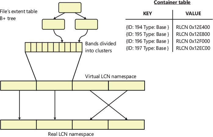
Figure 11-92 The container table provides a virtual LCN-to-real LCN indirection layer.

The container table is important: all the data managed by ReFS and Minstore needs to pass through the container table (with only small exceptions), so ReFS maintains multiple copies of this vital table. To perform an I/O on a block, ReFS must first look up the location of the extent’s container to find the real location of the data. This is achieved through the extent table, which contains target virtual LCN of the cluster range in the data section of its rows. The container ID is derived from the LCN, through a mathematical relationship. The new level of indirection allows ReFS to move the location of containers without consulting or modifying the file extent tables.

ReFS consumes tiers produced by Storage Spaces, hardware tiered volumes, and SMR disks. ReFS redirects small random I/Os to a portion of the faster tiers and destages those writes in batches to the slower tiers using sequential writes (destages happen at container granularity). Indeed, in ReFS, the term fast tier (or flash tier) refers to the random-access zone, which might be provided by the conventional bands of an SMR disk, or by the totality of an SSD or NVMe device. The term slow tier (or HDD tier) refers instead to the sequential write bands or to a rotating disk. ReFS uses different behaviors based on the class of the underlying medium. Non-SMR disks have no sequential requirements, so clusters can be allocated from anywhere on the volume; SMR disks, as discussed previously, need to have strictly sequential requirements, so ReFS never writes random data on the slow tier.

By default, all of the metadata that ReFS uses needs to stay in the fast tier; ReFS tries to use the fast tier even when processing general write requests. In non-SMR disks, as flash containers fill, ReFS moves containers from flash to HDD (this means that in a continuous write workload, ReFS is continually moving containers from flash into HDD). ReFS is also able to do the opposite when needed—select containers from the HDD and move them into flash to fill with subsequent writes. This feature is called container rotation and is implemented in two stages. After the storage driver has copied the actual data, ReFS modifies the container LCN mapping shown earlier. No modification in any file’s extent table is needed.

Container rotation is implemented only for non-SMR disks. This is important, because in SMR disks, the ReFS file system driver never automatically moves data between tiers. Applications that are SMR disk–aware and want to write data in the SMR capacity tier can use the FSCTL_SET_REFS_FILE_STRICTLY_SEQUENTIAL control code. If an application sends the control code on a file handle, the ReFS driver writes all of the new data in the capacity tier of the volume.

EXPERIMENT: Witnessing SMR disk tiers

You can use the FsUtil tool, which is provided by Windows, to query the information of an SMR disk, like the size of each tier, the usable and free space, and so on. To do so, just run the tool in an administrative command prompt. You can launch the command prompt as administrator by searching for cmd in the Cortana Search box and by selecting Run As Administrator after right-clicking the Command Prompt label. Input the following parameters:

Click here to view code image

fsutil volume smrInfo <VolumeDrive>

replacing the <VolumeDrive> part with the drive letter of your SMR disk.

Furthermore, you can start a garbage collection (see the next paragraph for details about this feature) through the following command:

Click here to view code image

fsutil volume smrGc <VolumeDrive> Action=startfullspeed

The garbage collection can even be stopped or paused through the relative Action parameter. You can start a more precise garbage collection by specifying the IoGranularity parameter, which specifies the granularity of the garbage collection I/O, and using the start action instead of startfullspeed.

Container compaction

Container rotation has performance problems, especially when storing small files that don’t usually fit into an entire band. Furthermore, in SMR disks, container rotation is never executed, as we explained earlier. Recall that each SMR band has an associated write pointer (hardware implemented), which identifies the location for sequential writing. If the system were to write before or after the write pointer in a non-sequential way, it would corrupt data located in other clusters (the SMR firmware must therefore refuse such a write).

ReFS supports two types of containers: base containers, which map a virtual cluster’s range directly to physical space, and compacted containers, which map a virtual container to many different base containers. To correctly map the correspondence between the space mapped by a compacted container and the base containers that compose it, ReFS implements an allocation bitmap, which is stored in the rows of the global container index table (another table, in which every row describes a single compacted container). The bitmap has a bit set to 1 if the relative cluster is allocated; otherwise, it’s set to 0.

Figure 11-93 shows an example of a base container (C32) that maps a range of virtual LCNs (0x8000 to 0x8400) to real volume’s LCNs (0xB800 to 0xBC00, identified by R46). As previously discussed, the container ID of a given virtual LCN range is derived from the starting virtual cluster number; all the containers are virtually contiguous. In this way, ReFS never needs to look up a container ID for a given container range. Container C32 of Figure 11-93 only has 560 clusters (0x230) contiguously allocated (out of its 1,024). Only the free space at the end of the base container can be used by ReFS. Or, for non-SMR disks, in case a big chunk of space located in the middle of the base container is freed, it can be reused too. Even for non-SMR disks, the important requirement here is that the space must be contiguous.

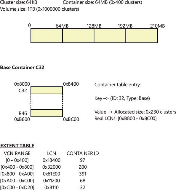
Figure 11-93 An example of a base container addressed by a 210 MB file. Container C32 uses only 35 MB of its 64 MB space.

If the container becomes fragmented (because some small file extents are eventually freed), ReFS can convert the base container into a compacted container. This operation allows ReFS to reuse the container’s free space, without reallocating any row in the extent table of the files that are using the clusters described by the container itself.

ReFS provides a way to defragment containers that are fragmented. During normal system I/O activity, there are a lot of small files or chunks of data that need to be updated or created. As a result, containers located in the slow tier can hold small chunks of freed clusters and can become quickly fragmented. Container compaction is the name of the feature that generates new empty bands in the slow tier, allowing containers to be properly defragmented. Container compaction is executed only in the capacity tier of a tiered volume and has been designed with two different goals:

• ■    Compaction is the garbage collector for SMR-disks: In SMR, ReFS can only write data in the capacity zone in a sequential manner. Small data can’t be singularly updated in a container located in the slow tier. The data doesn’t reside at the location pointed by the SMR write pointer, so any I/O of this kind can potentially corrupt other data that belongs to the band. In that case, the data is copied in a new band. Non-SMR disks don’t have this problem; ReFS updates data residing in the small tier directly.

• ■    In non-SMR tiered volumes, compaction is the generator for container rotation: The generated free containers can be used as targets for forward rotation when data is moved from the fast tier to the slow tier.

ReFS, at volume-format time, allocates some base containers from the capacity tier just for compaction; which are called compacted reserved containers. Compaction works by initially searching for fragmented containers in the slow tier. ReFS reads the fragmented container in system memory and defragments it. The defragmented data is then stored in a compacted reserved container, located in the capacity tier, as described above. The original container, which is addressed by the file extent table, becomes compacted. The range that describes it becomes virtual (compaction adds another indirection layer), pointing to virtual LCNs described by another base container (the reserved container). At the end of the compaction, the original physical container is marked as freed and is reused for different purposes. It also can become a new compacted reserved container. Because containers located in the slow tier usually become highly fragmented in a relatively small time, compaction can generate a lot of empty bands in the slow tier.

The clusters allocated by a compacted container can be stored in different base containers. To properly manage such clusters in a compacted container, which can be stored in different base containers, ReFS uses another extra layer of indirection, which is provided by the global container index table and by a different layout of the compacted container. Figure 11-94 shows the same container as Figure 11-93, which has been compacted because it was fragmented (272 of its 560 clusters have been freed). In the container table, the row that describes a compacted container stores the mapping between the cluster range described by the compacted container, and the virtual clusters described by the base containers. Compacted containers support a maximum of four different ranges (called legs). The four legs create the second indirection layer and allow ReFS to perform the container defragmentation in an efficient way. The allocation bitmap of the compacted container provides the second indirection layer, too. By checking the position of the allocated clusters (which correspond to a 1 in the bitmap), ReFS is able to correctly map each fragmented cluster of a compacted container.

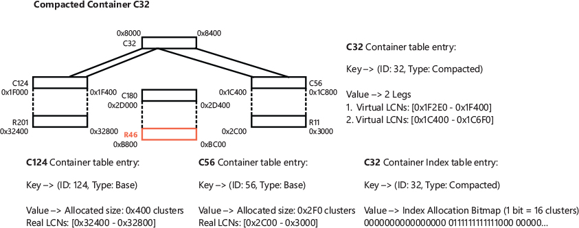
Figure 11-94 Container C32 has been compacted in base container C124 and C56.

In the example in Figure 11-94, the first bit set to 1 is at position 17, which is 0x11 in hexadecimal. In the example, one bit corresponds to 16 clusters; in the actual implementation, though, one bit corresponds to one cluster only. This means that the first cluster allocated at offset 0x110 in the compacted container C32 is stored at the virtual cluster 0x1F2E0 in the base container C124. The free space available after the cluster at offset 0x230 in the compacted container C32, is mapped into base container C56. The physical container R46 has been remapped by ReFS and has become an empty compacted reserved container, mapped by the base container C180.

In SMR disks, the process that starts the compaction is called garbage collection. For SMR disks, an application can decide to manually start, stop, or pause the garbage collection at any time through the FSCTL_SET_REFS_SMR_VOLUME_GC_PARAMETERS file system control code.

In contrast to NTFS, on non-SMR disks, the ReFS volume analysis engine can automatically start the container compaction process. ReFS keeps track of the free space of both the slow and fast tier and the available writable free space of the slow tier. If the difference between the free space and the available space exceeds a threshold, the volume analysis engine kicks off and starts the compaction process. Furthermore, if the underlying storage is provided by Storage Spaces, the container compaction runs periodically and is executed by a dedicated thread.

Compression and ghosting

ReFS does not support native file system compression, but, on tiered volumes, the file system is able to save more free containers on the slow tier thanks to container compression. Every time ReFS performs container compaction, it reads in memory the original data located in the fragmented base container. At this stage, if compression is enabled, ReFS compresses the data and finally writes it in a compressed compacted container. ReFS supports four different compression algorithms: LZNT1, LZX, XPRESS, and XPRESS_HUFF.

Many hierarchical storage management (HMR) software solutions support the concept of a ghosted file. This state can be obtained for many different reasons. For example, when the HSM migrates the user file (or some chunks of it) to a cloud service, and the user later modifies the copy located in the cloud through a different device, the HSM filter driver needs to keep track of which part of the file changed and needs to set the ghosted state on each modified file’s range. Usually HMRs keep track of the ghosted state through their filter drivers. In ReFS, this isn’t needed because the ReFS file system exposes a new I/O control code, FSCTL_GHOST_FILE_EXTENTS. Filter drivers can send the IOCTL to the ReFS driver to set part of the file as ghosted. Furthermore, they can query the file’s ranges that are in the ghosted state through another I/O control code: FSCTL_QUERY_GHOSTED_FILE_EXTENTS.

ReFS implements ghosted files by storing the new state information directly in the file’s extent table, which is implemented through an embedded table in the file record, as explained in the previous section. A filter driver can set the ghosted state for every range of the file (which must be cluster-aligned). When the ReFS driver intercepts a read request for an extent that is ghosted, it returns a STATUS_GHOSTED error code to the caller, which a filter driver can then intercept and redirect the read to the proper place (the cloud in the previous example).

Storage Spaces

Storage Spaces is the technology that replaces dynamic disks and provides virtualization of physical storage hardware. It has been initially designed for large storage servers but is available even in client editions of Windows 10. Storage Spaces also allows the user to create virtual disks composed of different underlying physical mediums. These mediums can have different performance characteristics.

At the time of this writing, Storage Spaces is able to work with four types of storage devices: Nonvolatile memory express (NVMe), flash disks, persistent memory (PM), SATA and SAS solid state drives (SSD), and classical rotating hard-disks (HDD). NVMe is considered the faster, and HDD is the slowest. Storage spaces was designed with four goals:

• ■    Performance: Spaces implements support for a built-in server-side cache to maximize storage performance and support for tiered disks and RAID 0 configuration.

• ■    Reliability: Other than span volumes (RAID 0), spaces supports Mirror (RAID 1 and 10) and Parity (RAID 5, 6, 50, 60) configurations when data is distributed through different physical disks or different nodes of the cluster.

• ■    Flexibility: Storage spaces allows the system to create virtual disks that can be automatically moved between a cluster’s nodes and that can be automatically shrunk or extended based on real space consumption.

• ■    Availability: Storage spaces volumes have built-in fault tolerance. This means that if a drive, or even an entire server that is part of the cluster, fails, spaces can redirect the I/O traffic to other working nodes without any user intervention (and in a way). Storage spaces don’t have a single point of failure.

Storage Spaces Direct is the evolution of the Storage Spaces technology. Storage Spaces Direct is designed for large datacenters, where multiple servers, which contain different slow and fast disks, are used together to create a pool. The previous technology didn’t support clusters of servers that weren’t attached to JBOD disk arrays; therefore, the term direct was added to the name. All servers are connected through a fast Ethernet connection (10GBe or 40GBe, for example). Presenting remote disks as local to the system is made possible by two drivers—the cluster miniport driver (Clusport.sys) and the cluster block filter driver (Clusbflt.sys)—which are outside the scope of this chapter. All the storage physical units (local and remote disks) are added to a storage pool, which is the main unit of management, aggregation, and isolation, from where virtual disks can be created.

The entire storage cluster is mapped internally by Spaces using an XML file called BluePrint. The file is automatically generated by the Spaces GUI and describes the entire cluster using a tree of different storage entities: Racks, Chassis, Machines, JBODs (Just a Bunch of Disks), and Disks. These entities compose each layer of the entire cluster. A server (machine) can be connected to different JBODs or have different disks directly attached to it. In this case, a JBOD is abstracted and represented only by one entity. In the same way, multiple machines might be located on a single chassis, which could be part of a server rack. Finally, the cluster could be made up of multiple server racks. By using the Blueprint representation, Spaces is able to work with all the cluster disks and redirect I/O traffic to the correct replacement in case a fault on a disk, JBOD, or machine occurs. Spaces Direct can tolerate a maximum of two contemporary faults.

Spaces internal architecture

One of the biggest differences between Spaces and dynamic disks is that Spaces creates virtual disk objects, which are presented to the system as actual disk device objects by the Spaces storage driver (Spaceport.sys). Dynamic disks operate at a higher level: virtual volume objects are exposed to the system (meaning that user mode applications can still access the original disks). The volume manager is the component responsible for creating the single volume composed of multiple dynamic volumes. The Storage Spaces driver is a filter driver (a full filter driver rather than a minifilter) that lies between the partition manager (Partmgr.sys) and the disk class driver.

Storage Spaces architecture is shown in Figure 11-95 and is composed mainly of two parts: a platform-independent library, which implements the Spaces core, and an environment part, which is platform-dependent and links the Spaces core to the current environment. The Environment layer provides to Storage Spaces the basic core functionalities that are implemented in different ways based on the platform on which they run (because storage spaces can be used as bootable entities, the Windows boot loader and boot manager need to know how to parse storage spaces, hence the need for both a UEFI and Windows implementation). The core basic functionality includes memory management routines (alloc, free, lock, unlock and so on), device I/O routines (Control, Pnp, Read, and Write), and synchronization methods. These functions are generally wrappers to specific system routines. For example, the read service, on Windows platforms, is implemented by creating an IRP of type IRP_MJ_READ and by sending it to the correct disk driver, while, on UEFI environments, it’s implemented by using the BLOCK_IO_PROTOCOL.

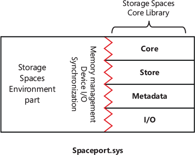
Figure 11-95 Storage Spaces architecture.

Other than the boot and Windows kernel implementation, storage spaces must also be available during crash dumps, which is provided by the Spacedump.sys crash dump filter driver. Storage Spaces is even available as a user-mode library (Backspace.dll), which is compatible with legacy Windows operating systems that need to operate with virtual disks created by Spaces (especially the VHD file), and even as a UEFI DXE driver (HyperSpace.efi), which can be executed by the UEFI BIOS, in cases where even the EFI System Partition itself is present on a storage space entity. Some new Surface devices are sold with a large solid-state disk that is actually composed of two or more fast NVMe disks.

Spaces Core is implemented as a static library, which is platform-independent and is imported by all of the different environment layers. Is it composed of four layers: Core, Store, Metadata, and IO. The Core is the highest layer and implements all the services that Spaces provides. Store is the component that reads and writes records that belong to the cluster database (created from the BluePrint file). Metadata interprets the binary records read by the Store and exposes the entire cluster database through different objects: Pool, Drive, Space, Extent, Column, Tier, and Metadata. The IO component, which is the lowest layer, can emit I/Os to the correct device in the cluster in the proper sequential way, thanks to data parsed by higher layers.

Services provided by Spaces

Storage Spaces supports different disk type configurations. With Spaces, the user can create virtual disks composed entirely of fast disks (SSD, NVMe, and PM), slow disks, or even composed of all four supported disk types (hybrid configuration). In case of hybrid deployments, where a mix of different classes of devices are used, Spaces supports two features that allow the cluster to be fast and efficient:

• ■    Server cache: Storage Spaces is able to hide a fast drive from the cluster and use it as a cache for the slower drives. Spaces supports PM disks to be used as a cache for NVMe or SSD disks, NVMe disks to be used as cache for SSD disks, and SSD disks to be used as cache for classical rotating HDD disks. Unlike tiered disks, the cache is invisible to the file system that resides on the top of the virtual volume. This means that the cache has no idea whether a file has been accessed more recently than another file. Spaces implements a fast cache for the virtual disk by using a log that keeps track of hot and cold blocks. Hot blocks represent parts of files (files’ extents) that are often accessed by the system, whereas cold blocks represent part of files that are barely accessed. The log implements the cache as a queue, in which the hot blocks are always at the head, and cold blocks are at the tail. In this way, cold blocks can be deleted from the cache if it’s full and can be maintained only on the slower storage; hot blocks usually stay in the cache for a longer time.

• ■    Tiering: Spaces can create tiered disks, which are managed by ReFS and NTFS. Whereas ReFS supports SMR disks, NTFS only supports tiered disks provided by Spaces. The file system keeps track of the hot and cold blocks and rotates the bands based on the file’s usage (see the “ReFS support for tiered volumes and SMR” section earlier in this chapter). Spaces provides to the file system driver support for pinning, a feature that can pin a file to the fast tier and lock it in the tier until it will be unpinned. In this case, no band rotation is ever executed. Windows uses the pinning feature to store the new files on the fast tier while performing an OS upgrade.

As already discussed previously, one of the main goals of Storage Spaces is flexibility. Spaces supports the creation of virtual disks that are extensible and consume only allocated space in the underlying cluster’s devices; this kind of virtual disk is called thin provisioned. Unlike fixed provisioned disks, where all of the space is allocated to the underlying storage cluster, thin provisioned disks allocate only the space that is actually used. In this way, it’s possible to create virtual disks that are much larger than the underlying storage cluster. When available space gets low, a system administrator can dynamically add disks to the cluster. Storage Spaces automatically includes the new physical disks to the pool and redistributes the allocated blocks between the new disks.

Storage Spaces supports thin provisioned disks through slabs. A slab is a unit of allocation, which is similar to the ReFS container concept, but applied to a lower-level stack: the slab is an allocation unit of a virtual disk and not a file system concept. By default, each slab is 256 MB in size, but it can be bigger in case the underlying storage cluster allows it (i.e., if the cluster has a lot of available space.) Spaces core keeps track of each slab in the virtual disk and can dynamically allocate or free slabs by using its own allocator. It’s worth noting that each slab is a point of reliability: in mirrored and parity configurations, the data stored in a slab is automatically replicated through the entire cluster.

When a thin provisioned disk is created, a size still needs to be specified. The virtual disk size will be used by the file system with the goal of correctly formatting the new volume and creating the needed metadata. When the volume is ready, Spaces allocates slabs only when new data is actually written to the disk—a method called allocate-on-write. Note that the provisioning type is not visible to the file system that resides on top of the volume, so the file system has no idea whether the underlying disk is thin or fixed provisioned.

Spaces gets rid of any single point of failure by making usage of mirroring and pairing. In big storage clusters composed of multiple disks, RAID 6 is usually employed as the parity solution. RAID 6 allows the failure of a maximum of two underlying devices and supports seamless reconstruction of data without any user intervention. Unfortunately, when the cluster encounters a single (or double) point of failure, the time needed to reconstruct the array (mean time to repair or MTTR) is high and often causes serious performance penalties.

Spaces solves the problem by using a local reconstruction code (LCR) algorithm, which reduces the number of reads needed to reconstruct a big disk array, at the cost of one additional parity unit. As shown in Figure 11-96, the LRC algorithm does so by dividing the disk array in different rows and by adding a parity unit for each row. If a disk fails, only the other disks of the row needs to be read. As a result, reconstruction of a failed array is much faster and more efficient.

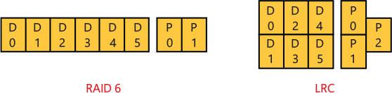
Figure 11-96 RAID 6 and LRC parity.

Figure 11-96 shows a comparison between the typical RAID 6 parity implementation and the LRC implementation on a cluster composed of eight drives. In the RAID 6 configuration, if one (or two) disk(s) fail(s), to properly reconstruct the missing information, the other six disks need to be read; in LRC, only the disks that belong to the same row of the failing disk need to be read.

EXPERIMENT: Creating tiered volumes

Storage Spaces is supported natively by both server and client editions of Windows 10. You can create tiered disks using the graphical user interface, or you can also use Windows PowerShell. In this experiment, you will create a virtual tiered disk, and you will need a workstation that, other than the Windows boot disk, also has an empty SSD and an empty classical rotating disk (HDD). For testing purposes, you can emulate a similar configuration by using HyperV. In that case, one virtual disk file should reside on an SSD, whereas the other should reside on a classical rotating disk.

First, you need to open an administrative Windows PowerShell by right-clicking the Start menu icon and selecting Windows PowerShell (Admin). Verify that the system has already identified the type of the installed disks:

Click here to view code image

PS C:\> Get-PhysicalDisk | FT DeviceId, FriendlyName, UniqueID, Size, MediaType, CanPool
    
    DeviceId FriendlyName            UniqueID                      Size MediaType CanPool
    -------- ------------            --------                      ---- --------- -------
    2        Samsung SSD 960 EVO 1TB eui.0025385C61B074F7 1000204886016 SSD         False
    0        Micron 1100 SATA 512GB  500A071516EBA521      512110190592 SSD         True
    1        TOSHIBA DT01ACA200      500003F9E5D69494     2000398934016 HDD         True

In the preceding example, the system has already identified two SSDs and one classical rotating hard disk. You should verify that your empty disks have the CanPool value set to True. Otherwise, it means that the disk contains valid partitions that need to be deleted. If you’re testing a virtualized environment, often the system is not able to correctly identify the media type of the underlying disk.

Click here to view code image

PS C:\> Get-PhysicalDisk | FT DeviceId, FriendlyName, UniqueID, Size, MediaType, CanPool
    
    DeviceId FriendlyName      UniqueID                                  Size MediaType   CanPool
    -------- ------------      --------                                  ---- ---------   -------
    2        Msft Virtual Disk 600224802F4EE1E6B94595687DDE774B  137438953472 Unspecified    True
    1        Msft Virtual Disk 60022480170766A9A808A30797285D77 1099511627776 Unspecified    True
    0        Msft Virtual Disk 6002248048976A586FE149B00A43FC73  274877906944 Unspecified   False

In this case, you should manually specify the type of disk by using the command Set-PhysicalDisk -UniqueId (Get-PhysicalDisk)[<IDX>].UniqueID -MediaType <Type>, where IDX is the row number in the previous output and MediaType is SSD or HDD, depending on the disk type. For example:

Click here to view code image

PS C:\> Set-PhysicalDisk -UniqueId (Get-PhysicalDisk)[0].UniqueID -MediaType SSD
    PS C:\> Set-PhysicalDisk -UniqueId (Get-PhysicalDisk)[1].UniqueID -MediaType HDD
    PS C:\> Get-PhysicalDisk | FT DeviceId, FriendlyName, UniqueID, Size, MediaType, CanPool
    
    DeviceId FriendlyName      UniqueID                                  Size MediaType   CanPool
    -------- ------------      --------                                  ---- ---------   -------
    2        Msft Virtual Disk 600224802F4EE1E6B94595687DDE774B  137438953472 SSD            True
    1        Msft Virtual Disk 60022480170766A9A808A30797285D77 1099511627776 HDD            True
    0        Msft Virtual Disk 6002248048976A586FE149B00A43FC73  274877906944 Unspecified   False

At this stage you need to create the Storage pool, which is going to contain all the physical disks that are going to compose the new virtual disk. You will then create the storage tiers. In this example, we named the Storage Pool as DefaultPool:

Click here to view code image

PS C:\> New-StoragePool -StorageSubSystemId (Get-StorageSubSystem).UniqueId -FriendlyName
    DeafultPool -PhysicalDisks (Get-PhysicalDisk -CanPool $true)
    
    FriendlyName OperationalStatus HealthStatus IsPrimordial IsReadOnly    Size AllocatedSize
    ------------ ----------------- ------------ ------------ ----------    ---- -------------
    Pool         OK                Healthy      False             1.12 TB        512 MB
    
    
    PS C:\> Get-StoragePool DefaultPool | New-StorageTier -FriendlyName SSD -MediaType SSD
    ...
    PS C:\> Get-StoragePool DefaultPool | New-StorageTier -FriendlyName HDD -MediaType HDD
    ...

Finally, we can create the virtual tiered volume by assigning it a name and specifying the correct size of each tier. In this example, we create a tiered volume named TieredVirtualDisk composed of a 120-GB performance tier and a 1,000-GB capacity tier:

Click here to view code image

PS C:\> $SSD = Get-StorageTier -FriendlyName SSD
    PS C:\> $HDD = Get-StorageTier -FriendlyName HDD
    PS C:\> Get-StoragePool Pool | New-VirtualDisk -FriendlyName "TieredVirtualDisk"
    -ResiliencySettingName "Simple" -StorageTiers $SSD, $HDD -StorageTierSizes 128GB, 1000GB
    ...
    PS C:\> Get-VirtualDisk | FT FriendlyName, OperationalStatus, HealthStatus, Size,
    FootprintOnPool
    
    FriendlyName      OperationalStatus HealthStatus          Size FootprintOnPool
    ------------      ----------------- ------------          ---- ---------------
    TieredVirtualDisk OK                Healthy      1202590842880   1203664584704

After the virtual disk is created, you need to create the partitions and format the new volume through standard means (such as by using the Disk Management snap-in or the Format tool). After you complete volume formatting, you can verify whether the resulting volume is really a tiered volume by using the fsutil.exe tool:

Click here to view code image

PS E:\> fsutil tiering regionList e:
    Total Number of Regions for this volume: 2
    Total Number of Regions returned by this operation: 2
    
       Region # 0:
            Tier ID: {448ABAB8-F00B-42D6-B345-C8DA68869020}
            Name: TieredVirtualDisk-SSD
            Offset: 0x0000000000000000
            Length: 0x0000001dff000000
    
       Region # 1:
            Tier ID: {16A7BB83-CE3E-4996-8FF3-BEE98B68EBE4}
            Name: TieredVirtualDisk-HDD
            Offset: 0x0000001dff000000
            Length: 0x000000f9ffe00000

Conclusion

Windows supports a wide variety of file system formats accessible to both the local system and remote clients. The file system filter driver architecture provides a clean way to extend and augment file system access, and both NTFS and ReFS provide a reliable, secure, scalable file system format for local file system storage. Although ReFS is a relatively new file system, and implements some advanced features designed for big server environments, NTFS was also updated with support for new device types and new features (like the POSIX delete, online checkdisk, and encryption).

The cache manager provides a high-speed, intelligent mechanism for reducing disk I/O and increasing overall system throughput. By caching on the basis of virtual blocks, the cache manager can perform intelligent read-ahead, including on remote, networked file systems. By relying on the global memory manager’s mapped file primitive to access file data, the cache manager can provide a special fast I/O mechanism to reduce the CPU time required for read and write operations, while also leaving all matters related to physical memory management to the Windows memory manager, thus reducing code duplication and increasing efficiency.

Through DAX and PM disk support, storage spaces and storage spaces direct, tiered volumes, and SMR disk compatibility, Windows continues to be at the forefront of next-generation storage architectures designed for high availability, reliability, performance, and cloud-level scale.

In the next chapter, we look at startup and shutdown in Windows.